
J_Ecoacoust 2022, 6(1), 1; doi:10.35995/jea6010001
Article
A Suburban Soundscape Reveals Altered Acoustic Dynamics during the COVID-19 Lockdown
Samuel R.P.-J. Ross 1,2,*
1
Department of Zoology, School of Natural Sciences, Trinity College Dublin, Dublin 2, Ireland
2
Integrative Community Ecology (Armitage) Unit, Okinawa Institute of Science & Technology Graduate University,
1919-1 Tancha, Onna-son, Okinawa, 904-0495 Japan
*
Corresponding author: s.ross.res@outlook.com
How to cite: Ross, S.R.P.-J. A Suburban Soundscape Reveals Altered Acoustic Dynamics during the COVID-19 Lockdown. J. Ecoacoust. 2020, 6(1), 1; doi:10.35995/jea6010001.
Received: 2 November 2020 / Accepted: 31 May 2022 / Published: 7 November 2022
Abstract
:The 2020 COVID-19 pandemic and the resulting national and international movement restrictions provide a unique opportunity to investigate the consequences of changing anthropogenic noise regimes on animal communities and soundscapes. Here, I used this lockdown period as a natural experiment to investigate changes to soundscape intensity, structure, and dynamics during restricted human activity (lockdown) in suburban Nottingham, UK. Using 11 common acoustic indices, I tested for differences in the richness and evenness of the soundscape during the COVID-19 lockdown, and I measured changes in soundscape dynamics by comparing the temporal variability of acoustic indices during versus after the lockdown. Regardless of how the soundscape was summarised, there were significant differences in the intensity, evenness, and temporal variability of the soundscape during the COVID-19 lockdown, principally driven by changes to anthropogenic noise. I recorded a shift away from a dominance of anthropophony towards more intense biological sounds during the lockdown, and the lockdown soundscape was generally more even, particularly because of changes to the magnitude of the diurnal cycle. These preliminary results from a mass human confinement experiment provide an early glimpse into how suburban soundscapes are impacted by noise pollution. In time, globally distributed longer-term monitoring efforts will reveal the generality of these findings, facilitating a mechanistic understanding of the impacts of anthropogenic noise on the world’s natural and human-dominated soundscapes.
Keywords:
acoustic monitoring; acoustic index; soundscape variability; noise pollution; anthropophony; COVID-19; ecoacousticsIntroduction
Ecoacoustics—the ecological study of sound across spatial and temporal scales (Farina, 2018)—is increasingly used as a framework to understand how animal communities and soundscapes (sensu Pijanowski et al., 2011) are impacted by anthropogenic disturbance, including habitat destruction (Deichmann et al., 2017; Burivalova et al., 2018, 2019b; Gasc et al., 2018), urbanisation (Joo et al., 2011; Ross et al., 2018; Marín-Gómez et al., 2020), noise pollution (Francis et al., 2009; Barton et al., 2018; Senzaki et al., 2020; Duarte et al., 2021), and climate change (Narins and Meenderink, 2014; Krause and Farina, 2016; Sueur et al., 2019). The field makes use of passive acoustic monitoring methods and a suite of acoustic indices to rapidly summarise the soundscape, including biophony (biological sounds), geophony (e.g., wind, rain), and anthropophony (human-related sounds; Pijanowski et al., 2011). Many acoustic indices have been developed to date (reviewed in Sueur et al., 2014), each aiming to characterise a specific property of the soundscape (Bradfer-Lawrence et al., 2019), and each touted as relating to a useful aspect of biodiversity or landscape structure (Gasc et al., 2013; Fuller et al., 2015; Mammides et al., 2017; Buxton et al., 2018; Elise et al., 2019; Ross et al., 2021a). Briefly, these indices can be grouped into several classes. Richness or intensity indices generally represent the total ‘loudness’ of the soundscape at different frequencies, where acoustic energy in the primarily biotic frequency range (2 kHz) generally indicates a greater number (but not necessarily diversity) of animal vocalisations, while loudness in the 1–2 kHz range represents a stronger influence of anthropophony (Kasten et al., 2012). Evenness indices measure the distribution of acoustic energy across different frequency bins or time points within each recording (Pieretti et al., 2011; Villanueva-Rivera et al., 2011), where higher evenness may represent the saturation of the soundscape due to the high density of vocalisations (Fuller et al., 2015; Mammides et al., 2017; but see Bradfer-Lawrence et al., 2020). Finally, some indices (e.g., acoustic richness; Depraetere et al., 2012) consider both the intensity and evenness simultaneously. However, despite their utility as rapid indicators of soundscape conditions, we still lack mechanistic insight into the world’s soundscapes, in large part due to the challenge of accurately inferring driving processes from observational acoustic monitoring data.
One of the difficulties in attaining a mechanistic insight into human impacts on soundscapes is that anthropogenic disturbances rarely occur in isolation. Most ecosystems are simultaneously subject to anthropogenic threat complexes, comprising multiple interacting disturbances (Bowler et al., 2019). Particularly intertwined are the impacts of anthropogenic noise (anthropophony) and urbanisation per se on animal communities since human activity leaves a large sonic footprint on ecosystems (Warren et al., 2006; Francis et al., 2009; Barber et al., 2010; Duarte et al., 2021). The global COVID-19 pandemic and its associated reductions in human movement and activity provide an unprecedented opportunity to disentangle urban environments from their associated anthropophony (Derryberry et al., 2020; Diffenbaugh et al., 2020; Douglas et al., 2020; Saraswat and Saraswat, 2020). Dubbed, the Anthropause (Rutz et al., 2020), the COVID-19 restrictions (henceforth “lockdowns”) can be seen as a “global human confinement experiment” to investigate the impacts of human activity on ecosystems (Bates et al., 2020). There is early evidence, particularly in urban environments, that lockdowns have reduced air and water pollution (Bao and Zhang, 2020; Le Quéré et al., 2020; but see Zangari et al., 2020), have allowed native and invasive species to exploit temporary changes to disturbance regimes (Manenti et al., 2020), and behavioural plasticity in songbirds has led to higher performance songs, with birds taking advantage of the vacant acoustic space usually dominated by anthropophony (Derryberry et al., 2020). Whether such shifts in acoustic space use were commonplace across diverse urban and suburban soundscapes during the COVID-19 lockdown remains an open question.
Here, I used the national COVID-19 lockdown in the United Kingdom as a human confinement experiment to investigate the effects of changes in human activity and mobility on the intensity and dynamics of a suburban soundscape in Nottingham, UK. Lockdowns reduced motor vehicle traffic across the world (Le Quéré et al., 2020), in some cases resulting in a >50-year low for noise pollution (Derryberry et al., 2020). I anticipate that when comparing lockdown and post-lockdown suburban soundscapes, I will find a shift in the prevalence of anthropogenic noise, as summarised by acoustic indices. I also focus here on the variability of soundscapes through time, since temporal variability represents an important dimension of stability (e.g., Guiz et al., 2016; Ross et al., 2021b), which, in turn, can aid in the conservation and management of natural soundscapes and the vital ecosystem services they provide (Dumyahn and Pijanowski, 2011; Elise et al., 2019; Levenhagen et al., 2021). Currently, little is known about how human activity shapes soundscape variability (Rodriguez et al., 2014; Francomano et al., 2020)—particularly in urban areas (Joo et al., 2011)—despite the importance of soundscape dynamics for answering biogeographical questions (Lomolino et al., 2015) and in establishing baselines for developing soundscapes as disturbance indicators (Almeira and Guecha, 2019; Burivalova et al., 2018, 2019a; Gasc et al., 2018; Francomano et al., 2020). By comparing the intensity, evenness, and temporal variability of a suburban soundscape between two time periods including the UK national COVID-19 lockdown, I provide preliminary evidence of human impacts on soundscapes and their dynamics.
Methods
Study Location
This study was conducted in suburban Woodthorpe, in the borough of Gedling, Nottinghamshire County, UK. The recording site is in a suburban area, on a cul-de-sac with limited traffic, but is situated ~55 m from a heavily trafficked road, and ~85 m from a recreational ground with sports fields and a children’s outdoor play area. Immediately opposite the recording site (~10 m away) is a patch of undeveloped land overgrown with weeds, shrubs, and trees. The biotic component of this soundscape is dominated by insects and common British garden birds (pers. obs.), including Eurasian Blackbirds and other Thrushes (Turdus sp.), various species of small Passerine Tits (Paridae sp.), Sparrows (Passeridae sp.), and lower frequency biotic sounds produced by Common Wood Pigeons (Columba palumbus), and Eurasian Magpies (Pica pica). Red Foxes (Vulpes vulpes), domestic cats, and Common Pipistrelle Bats (Pipistrellus pipistrellus, ~45 kHz) also make infrequent contributions to the nocturnal soundscape, particularly during the late summer months. d. Anthropophony primarily constitutes traffic noise from the adjacent road, and voices of local residents and from the nearby recreational ground.
Acoustic Recording and Lockdown Measures
During each of the two recording periods, I installed an Audiomoth recorder (ver 1.1.0, Hill et al., 2018) in an IPX7 Waterproof case on a tree branch, ~1.4 m from ground level. The recorder gain was set to low (27.2 dB), and the sampling rate to 48 kHz. I did not apply any filters to audio recordings, nor did I remove potentially confounding weather noise (geophony) manually or automatically. The recording schedule was 1 min of recording every 10 min (recording duration: 60 s, sleep duration: 540 s), and the recordings were saved in a .WAV format. This schedule reduces battery expenditure without significantly compromising the ability to detect biological signals in records (Pieretti et al., 2015); however, the acoustic index variance is artificially inflated relative to continuous recording (Bradfer-Lawrence et al., 2019). Nevertheless, as I used the same recording schedule for all recordings, pairwise comparisons are valid.
I recorded for two periods in the summer/autumn of 2020; one towards the end of the full COVID-19 lockdown in Nottingham (May 25–Jun 1; henceforth lockdown period), and one after travel restrictions had been fully lifted, but social distancing was still in place (Sep 28–Oct 10; post-lockdown period). During the UK’s lockdown period (beginning 23 Mar 2020), people were encouraged to work from home if possible, and only “essential” workers were permitted to travel for work. To combat mental and physical health problems, the UK government relaxed the restrictions to allow “unlimited amounts” of outdoor exercise, but people were still not permitted to gather in groups, and non-essential businesses, including restaurants, pubs, and shops, remained closed. During the lockdown, Nottingham operated a reduced schedule of public transport. May 28 marked the final “clap for our carers” event, where people gathered on doorsteps at 20:00 once a week to clap and cheer in support of essential workers, and this event is present in my recordings as a broadband signal (Supporting Figure S1).
During the post-lockdown period, most of the above restrictions had been lifted. Many people were again commuting to work, and schools had returned for in-person activity. Compared with non-pandemic years, audible human activity was likely still reduced; however, as a benchmark for “business as usual”, the Sep 28-Oct 10 period makes a suitable dataset to which comparisons with the full lockdown restrictions can be made. The post-lockdown period includes ~2 days (03 Oct 10:00–05 Oct 17:00) of missing data due to recorder failure. See Figure S2 for the spectrograms of typical lockdown and post-lockdown soundscapes.
Acoustic Indices
Using the seewave (ver 2.1.6, Sueur et al., 2008a) and soundecology (ver 1.3.3, Villanueva-Rivera and Pijanowski, 2018) packages in R (ver 4.0.2, R Core Team, 2020), I calculated 11 commonly used acoustic indices on each 1 min audio file (n = 2343). These were acoustic complexity (ACI, Pieretti et al., 2011); acoustic diversity (ADiv), and evenness (AEve, Villanueva-Rivera et al., 2011); the bioacoustic index (BioA, Boelman et al., 2007); the median of the amplitude envelope (M) and acoustic richness (ARic, Depraetere et al., 2012); the acoustic entropy (H) and temporal entropy (Ht) indices (Sueur et al., 2008b); and the normalised difference soundscape index (NDSI), including its two component indices biophony (NDSIBio), calculated as the intensity of the 2–11 kHz frequency range, and anthropophony (NDSIAnthro) which measures the intensity in the 1–2 kHz range (Kasten et al., 2012). In this way, NDSIBio and NDSIAnthro approximate the sound levels of the biophonic and anthropophonic components of the soundscape, respectively. For further details of acoustic index calculation, including their implementation in R, see Ross et al. (2021a).
Statistical Analysis
To test for differences in acoustic index values between the lockdown and post-lockdown periods, I used paired Wilcoxon signed rank tests. These are non-parametric tests and so make few assumptions regarding the data distribution, and they can handle uneven sample sizes between paired time periods. I tested for differences between all acoustic index values for each acoustic index during (n = 964) versus post-lockdown (n = 1379) and took the 95% confidence intervals around the difference to measure the standardised effect size. If the difference values ± 95% C.I.s did not span zero, the differences were regarded as significant (as also indicated by the Wilcoxon test p-value and associated Z-score). In all cases, I first scaled the acoustic indices by dividing them by their maximum before inclusion in the models (Bradfer-Lawrence et al., 2020). For the NDSI, which is bounded from −1 to 1, I scaled the values using (NDSI + 1)/2 (Fairbrass et al., 2017).
As these comparisons potentially include the confounding effects of time-of-day, I also tested for lockdown versus post-lockdown differences on various subsets of the data, again using paired Wilcoxon signed rank tests to make comparisons. These subsets included a seasonally adjusted dawn chorus (the hour including sunrise on a particular date), the hour of peak commuter travel time (08:00–09:00), and one hour each at midday (12:00–13:00) and midnight (00:00–01:00), aiming at capturing an average soundscape during daytime and night-time hours, respectively. Note that the northern latitudinal changes in day length produce seasonally adjusted dawn chorus times that differ between lockdown periods (for example, sunrise is 03:51 on May 25, but 06:20 on Oct 09). Therefore, to separate any seasonal artifacts in comparisons of the dawn chorus, I also tested for differences based only on the hour between 06:00 and 07:00.
To test for the effects of lockdown on soundscape dynamics, I also measured the temporal variability of each index, for all the available data and for each of the above subsets. I used the mean and standard deviation of the absolute model residuals of a generalised linear model (GLM) of acoustic index values against time as my measure of temporal variability and error, respectively (Guiz et al., 2016). In all cases, the GLMs were fitted with the “logit” link function and beta error distribution, which can accommodate the skewed data of acoustic indices, and can handle 0–1 standardised acoustic index values (Bradfer-Lawrence et al., 2020; Ross et al., 2021a). I used the mean (), standard deviation (), and sample size () of the absolute model residuals to produce the estimates of standardised effect sizes (SES) for the difference between lockdown periods, using the equation , where subscripts 1 and 2 represent the lockdown and post-lockdown periods, respectively. The critical z value () was set at 1.96 to produce 95% confidence intervals around the difference between lockdown periods. Where 95% confidence intervals did not span zero, I interpreted this as a significant difference between the lockdown and post-lockdown periods for the temporal variability of a given acoustic index. All the analyses were conducted in R (ver 4.0.2, R Core Team, 2020) using the Stats (ver 4.0.2) and glmmTMB (ver 1.0.2.1, Brooks et al., 2017) packages.
Results
Of the 11 acoustic indices I calculated, 6 of them were most notably different between the lockdown and post-lockdown periods overall. The normalised difference soundscape index (NDSI), and its component indices biophony (NDSIBio) and anthropophony (NDSIAnthro) differed between the lockdown periods (Figure 1), indicating a shift in the relative acoustic power of the biophony-dominated (2–11 kHz) versus the anthropophony-dominated frequency bins (1–2 kHz). Specifically, I found that the NDSI was significantly higher during lockdown (Lockdown = 0.6 ± 0.19 (Median ± S.D.), Post-lockdown = 0.44 ± 0.22, Wilcoxon: Z-score = 11.1, p < 0.001), as was NDSIBio (Lockdown = 0.4 ± 0.23, Post-lockdown = 0.27 ± 0.27, Z = 6.72, p < 0.001; Figure 2a). NDSIAnthro showed the opposite pattern, with lower values overall during the lockdown (Lockdown = 0.79 ± 0.25, Post-lockdown = 0.95 ± 0.19, Z = −12.6, p < 0.001; Figure 2a). Acoustic evenness (AEve), the bioacoustic index (BioA), and acoustic richness (ARic) also showed significant differences between the lockdown periods (Figure 3). Despite similar median values between the two time periods (Lockdown = 0.04 ± 0.22, Post-lockdown = 0.04 ± 0.19), AEve was significantly higher during the lockdown period (Z = 2.96, p = 0.003, Figure 2a); a pattern driven by the differences in the spread of the data (Figure S3). The related bioacoustic index was also higher during the lockdown (Lockdown = 0.17 ± 0.13, Post-lockdown = 0.12 ± 0.09, Z = 12, p < 0.001; Figure 2a), while ARic was significantly lower during the lockdown (Lockdown = 0.11 ± 0.1, Post-lockdown = 0.19 ± 0.16, Z = −14.1, p < 0.001; Figure 2a).
Figure 1.
COVID-19 lockdown affects the intensity of biophony and anthropophony. Radar plots show acoustic index values (scaled 0–1) for the normalised difference soundscape index (NDSI; a,d), biophony (NDSIBio; b,e), and anthropophony (NDSIAnthro; c,f) during the lockdown period (May 25–Jun 01; a–c) and the post-lockdown period (Sep 29-Oct 09; d–f). Individual boxes represent index values at 10 min resolution, where time is represented as a 24 h clock and dates progress outwards from the centre.
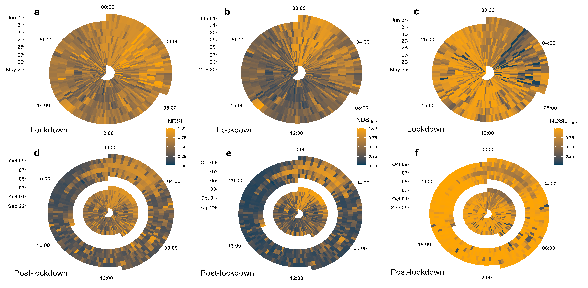
Figure 2.
Standardised effect sizes for the difference between lockdown and post-lockdown acoustic indices. Values represent standardised effect sizes calculated based on the difference between post-lockdown and lockdown periods for (a) 11 acoustic index values, and (b) the temporal variability in 11 acoustic indices, across all times. Note that these are comparisons of post-lockdown “business as usual” to the lockdown period, so effect sizes above zero represent an increase in acoustic index values (a) or an increase in temporal variability (b) during the lockdown period. Values which do not span zero (circles) are considered significant, while values spanning zero (triangles) do not differ significantly between post-lockdown and lockdown periods.
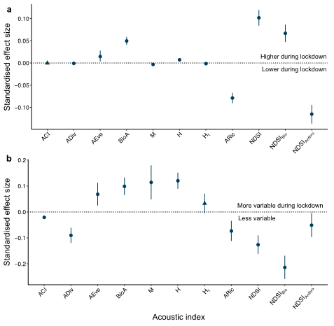
Figure 3.
COVID-19 lockdown affects soundscape evenness. Radar plots show acoustic index values (scaled 0–1) for acoustic evenness (AEve; a,d), the bioacoustic index (BioA; b,e), and acoustic richness (ARic; c,f) during the lockdown period (May 25-Jun 01; a–c) and the post-lockdown period (Sep 29-Oct 09; d–f). Individual boxes represent index values at 10 min resolution, where time is represented as a 24 h clock and dates progress outwards from the centre.
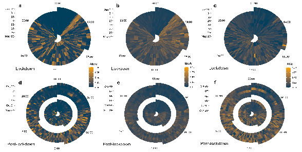
During the lockdown, the diurnal cycle of the NDSI and NDSIBio appeared visually less distinct, while post-lockdown, NDSIAnthro was close to its peak value for most of the 24 h cycle, showing only limited evidence that human activity is primarily restricted to daylight hours (Figure 1). For all these indices, there were significant differences between lockdown and post-lockdown in their values during the seasonally adjusted dawn chorus and the two morning periods (06:00 and 08:00). For example, NDSIBio was higher during the lockdown when considering the dawn chorus (Lockdown = 0.56 ± 0.15, Post-lockdown = 0.22 ± 0.18, Z = 4.88, p < 0.001), while anthropophony (NDSIAnthro) was less intense during the peak commuting time in the lockdown period (Lockdown = 0.75 ± 0.29, Post-lockdown = 0.96 ± 0.21, Z = -3.43, p < 0.001; Figure 4). However, these indices did not differ significantly between the lockdown periods when considering a standard daytime or night-time hour (Figure 4). The indices aimed at capturing evenness (AEve and BioA) showed clearer effects of the diurnal cycle during the lockdown, with a distinctive early morning (~3:00) dawn chorus during the lockdown (Figure 3a,b). Indeed, for the seasonally adjusted dawn chorus, both AEve (Lockdown = 0.41 ± 0.24, Post-lockdown = 0.09 ± 0.26, Z = 2.26, p = 0.023) and BioA were higher during the lockdown (Lockdown = 0.38 ± 0.12, Post-lockdown = 0.19 ± 0.09, Z = 5.19, p < 0.001; Figure 4).
Figure 4.
Standardised effect sizes for the difference between lockdown and post-lockdown acoustic indices. Values represent standardised effect sizes calculated based on the difference between post-lockdown and lockdown periods for 11 acoustic index values for five temporal subsets of the full dataset: the seasonally adjusted dawn chorus (Dawn); 06:00–07:00 (6 a.m.); peak commuting time, 08:00–09:00 (8 a.m.); 12:00–13:00 (Midday); and 00:00–01:00 (Midnight). For details of time period subsetting, including justification, see Methods. Interpretation follows Figure 2a.
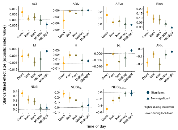
When considering the subsets of key hours, several indices consistently showed no difference between the lockdown periods (Figure 4). Acoustic complexity (ACI), diversity (ADiv), and evenness (AEve) did not differ between the lockdown periods for any of the hourly subsets excluding midnight and dawn (Figure 4), and the ACI was the only acoustic index not to differ significantly overall (Figure 2a). The Aric and the related median of the amplitude envelope (M) were both consistently lower during the lockdown regardless of the temporal subset considered (Figure 3c,f and Figure 4). The acoustic entropy (H) and temporal entropy (Ht) indices showed inverse patterns, with H increasing (Lockdown = 0.96 ± 0.03, Post-lockdown = 0.93 ± 0.02, Z = 2.49, p = 0.013) and Ht decreasing (Lockdown = 0.991 ± 0.01, Post-lockdown = 0.995 ± 0.01, Z = −2.34, p = 0.019) at 08:00–09:00 during the lockdown (Figure 4).
Temporal variability differed between the lockdown and post-lockdown periods for all indices but Ht (Figure 2b). When considering the whole dataset, four indices (AEve, BioA, M, and H) were more variable during the lockdown period, while most acoustic indices (ACI, Adiv, Aric, NDSI, NDSIBio, and NDSIAnthro) were less variable during the lockdown. The largest relative change in temporal variability when considering the whole time series was for NDSIBio (Lockdown = 0.76 ± 0.51 (residual Mean ± S.D.), Post-lockdown = 0.97 ± 0.58, SES range = −0.26–−0.17) which significantly differed from zero when quantified as the standardised effect size of the difference (Figure 2b). However, based on the hourly subsets, the variability of NDSIBio did not differ significantly between the lockdown periods at 8:00 or midnight (Figure S4).
Most acoustic indices did not differ significantly in their variability between the lockdown periods when considering the hourly subsets (Figure S4). BioA was not significantly different between the lockdown periods during any of the tested subsets, while five indices (ACI, Adiv, AEve, Ht, and NDSI) only differed during one hourly subset. Based on the standardised effect size of the difference, M was significantly less variable during the lockdown at the 06:00 (Lockdown = 0.13 ± 0.096, Post-lockdown = 0.23 ± 0.18, SES = −0.15–−0.04) and midnight (Lockdown = 0.055 ± 0.051, Post-lockdown = 0.57 ± 0.36, SES = −0.61–−0.43) subsets. NDSIBio and NDSIAnthro were both less variable during the lockdown for both the dawn chorus and 6:00 hourly subsets (Figure S4). Finally, H was the only index with consistently higher temporal variability during the lockdown regardless of the hourly subset considered (Figure S4), as also reflected by an overall higher temporal variability for the whole time series relative to the post-lockdown H values (Lockdown = 0.62 ± 0.38, Post-lockdown = 0.5 ± 0.36, SES = 0.09–0.15; Figure 2b).
Discussion
This study made use of the UK’s nationwide COVID-19 lockdown to infer the impacts of human activity on suburban soundscape dynamics. I compared the lockdown and post-lockdown values of acoustic indices and their temporal variability and found differences in the intensity, evenness, and variability of the soundscape during the COVID-19 lockdown. By viewing the COVID-19 movement restrictions as a human confinement experiment (Bates et al., 2020; Rutz et al., 2020), one can infer the impacts of anthropogenic activity on urban and suburban soundscapes. My results provide important early evidence that humans alter not only soundscape composition—as measured by several richness and evenness indices (Pieretti et al., 2011; Villanueva-Rivera et al., 2011; Depraetere et al., 2012)—but also the variability of soundscapes across multiple days.
Intuitively, anthropophony (NDSIAnthro) was lower and biophony (NDSIBio) higher during the lockdown compared with post-lockdown, suggesting a downward shift in the relative intensity of anthropogenic noise pollution during the lockdown (Derryberry et al., 2020; Ulloa et al., 2021). That biophony intensity differed between the lockdown periods suggests a plastic response of vocalising animals to the vacant acoustic space offered by human confinement. Though these analyses are insufficient to establish whether individual species respond through changes to song properties (e.g., frequency: Slabbekoorn and den Boer-Visser, 2006; Derryberry et al., 2020), more intense biophony during the lockdown suggests an increase in the activity and hence detectability of vocalising species, as reported for other cities during the lockdown (Estela et al., 2021; Gordo et al., 2021). Such a shift in activity patterns may also explain the observed differences in soundscape evenness in this system.
The soundscape was generally more even during the lockdown period, as quantified by acoustic evenness (AEve, Villanueva-Rivera et al., 2011) and the bioacoustic index (BioA, Boelman et al., 2007). This was the case on average when considering AEve and BioA across all one-minute recordings, as well as when considering early morning for BioA. While differences in evenness can reflect changes to the overall sound intensity (Shamon et al., 2021), most of the indices I used to measure soundscape richness or intensity (e.g., Aric and M) were not higher, and in fact were more often lower, during the lockdown. This means that observed differences in evenness are a function of the homogenisation of acoustic energy across frequency bins during the lockdown—a pattern supported by the reduced NDSIBio variability during the lockdown—implying higher richness and/or different composition of vocalising animal communities (Boelman et al., 2007; Villanueva-Rivera et al., 2011; Estela et al., 2021). Evenness indices also revealed a clearer differentiation between night and day during the COVID-19 lockdown, with higher evenness during daytime throughout lockdown (but see Bertucci et al., 2021), while the post-lockdown diurnal cycle was less distinct. This perhaps reflects a weakening in post-lockdown daytime soundscape evenness due to the resumption of human activity and its associated anthropophony. Indeed, anthropophony may be the main driver of differences in both the richness and evenness of soundscapes during the lockdown (Ulloa et al., 2021); where anthropophony decreased during the lockdown, soundscapes were less rich and more even. Note also that the night-time soundscape was less even than the daytime—a pattern attributed elsewhere to nocturnal insects (Almeira and Guecha, 2019; but see Francomano et al., 2020).
Two competing hypotheses exist regarding the relationship between biotic richness and soundscape evenness or variability. Firstly, higher avian species richness may contribute to less variable soundscapes due to saturation across frequency bins and through time (Fuller et al., 2015; Mammides et al., 2017). Alternatively, sites with a high richness and abundance of vocalising animals may be more variable, as acoustic energy is less evenly distributed among frequencies when multiple animals compete for acoustic space (Bradfer-Lawrence et al., 2020). These hypotheses primarily focus on evenness across frequency bins or temporal variability of a single sound file (e.g., Ht) but also serve as suitable hypotheses when considering variability through time as I do here. I found that most indices (with the notable exception of evenness measures and M) were less variable during the COVID-19 lockdown, suggesting that anthropogenic activity reduces the consistency and predictability of suburban soundscapes (Mazaris et al., 2009). These results support an earlier finding that biophony intensity is lower and variability higher in urban areas compared with other land cover types in Michigan, USA (Joo et al., 2011; see also Mazaris et al., 2009; Liu et al., 2013).
Acoustic temporal variability differs across ecosystems because of inherent differences in the multi-scale biotic drivers of ecological communities (Francomano et al., 2020). Uncovering the degree to which human land use and anthropophony decouple soundscape dynamics from habitat or landscape configuration is key to understanding the anthropogenic imprint on the dynamics of nature (Mazaris et al., 2009; Liu et al., 2013). Studying soundscape variability in urban and suburban areas during the Anthropause provides a unique opportunity to understand the consequences of noise pollution on the continued supply of the ecosystem services soundscapes provide (Elise et al., 2019; Levenhagen et al., 2021). Highly variable soundscapes may provide less consistent mental health benefits and ultimately lead to an “extinction of experience”, as continued urban intensification deepens the disconnect between people and nature (Gaston and Soga, 2020), and the COVID-19 pandemic may have long-lasting effects on how people perceive nature (Garrido-Cumbrera et al., 2021; Soga et al., 2021), including natural soundscapes. My finding of higher variability post-lockdown thus hints at a human-caused degradation of the consistency and stability of the essential mental health benefits and cultural values provided by soundscapes (Dumyahn and Pijanowski, 2011; Levenhagen et al., 2021).
This study is limited in scope by its opportunistic nature. The UK’s COVID-19 lockdown provided a rare opportunity to study the effects of human confinement on urban and suburban systems (Bates et al., 2020; Rutz et al., 2020), and establishing acoustic monitoring sites during the pandemic allows tracking the trajectory of soundscape change as urban areas return to “normal”. Ideally, to tease apart the confounding effects of seasonality on the soundscape, comparisons should be made to seasonally analogous pre-disturbance baselines (Derryberry et al., 2020; Rutz et al., 2020). However, where such long-term monitoring data is unavailable, it will be sufficient to carefully study the gradual return to the pre-lockdown levels of human mobility and its impacts on soundscapes. This study is also limited both by its scope, with roughly one week of data collection per period, and its inability to fully exclude the effects of seasonality when comparing lockdown and post-lockdown soundscapes. The timing of foraging, migration, and reproduction can cause seasonal changes to biophony (Towsey et al., 2014; Francomano et al., 2020), though the degree to which seasonality impacts soundscapes is site-specific (Krause et al., 2011; Lin et al., 2017). Seasonal change may also affect soundscape dynamics, with shifts away from birdsong—which is typically sporadic and transient in nature (Lin et al., 2017)—reducing temporal variability, particularly if replaced by broadband insect sounds (Farina et al., 2011). Though seasonality may have played a role in shaping the biophony results presented in this study, my observation of changes in anthropophony between the two periods is independent of seasonality. My results thus offer early insight into the potential impacts of human activity on suburban soundscapes.
Zangari et al. (2020) recently highlighted the importance of considering long-term trends in air pollution when investigating short-term changes during the COVID-19 lockdown. The same is true of changes to the soundscape. Certainly, soundscape dynamics should be considered within the context of their longer-term trends (Sueur et al., 2019; Francomano et al., 2020). To achieve such context, there must be a continued focus on the acoustic monitoring of ecosystems around the world in an effort to establish soundscape baselines (Pieretti et al., 2017; Almeira and Guecha, 2019; Deichmann et al., 2018; Ross et al., 2018; Burivalova et al., 2019a; Sugai, 2020). Only with such baselines can the impacts of climate change and other anthropogenic pressures on soundscapes be effectively quantified (Krause and Farina, 2016; Sueur et al., 2019; Derryberry et al., 2020; Marín-Gómez et al., 2020; Duarte et al., 2021). To do so requires a concerted effort to strengthen global collaborative networks despite the financial implications of the COVID-19 pandemic (Rutz et al., 2020; Zahawi et al., 2020). As researchers around the world begin to piece together the effects of the Anthropause on urban soundscapes, early results such as those presented here provide a valuable roadmap for answering questions about the human footprint on the world’s soundscapes.
Supplementary Materials
Data for analysis and all R code are available in the Zenodo digital repository http://doi.org/10.5281/zenodo.5170605 (Ross, 2021). Supporting Information: 4 supplementary figures (2 spectrogram figures (S1–S2), and 2 analyses (S3–S4)).
Author Contributions
SRP-JR conceived of and conducted all aspects of the study and wrote the manuscript for publication.
Funding
For the duration of this work, I was supported by an Irish Research Council postgraduate scholarship (Grant No. GOIPG/2018/3023).
Acknowledgments
My sincere thanks go to Colin and Georgina Anderson for their help remotely deploying the AudioMoth and storing data, Paula Tierney for helpful discussion, Hannah White and two anonymous reviewers for valuable comments on previous versions of this manuscript, and Almo Farina for his guidance and kindness throughout the review process. I would also like to acknowledge all the essential workers, particularly in the healthcare sector, who continue to work tirelessly to minimise the devastating impacts of the COVID-19 pandemic.
Conflicts of Interest
The author declares no conflicts of interest.
References
- Almeira, J.; Guecha, S. Dominant power spectrums as a tool to establish an ecoacoustic baseline in a premontane moist forest. Landscape and Ecological Engineering 2019, 15, 121–130. [Google Scholar] [CrossRef]
- Bao, R.; Zhang, A. Does lockdown reduce air pollution? Evidence from 44 cities in northern China. Science of the Total Environment 2020, 731, 139052. [Google Scholar] [CrossRef] [PubMed]
- Barber, J. R.; Crooks, K. R.; Fristrup, K. M. The costs of chronic noise exposure for terrestrial organisms. Trends in Ecology & Evolution 2010, 25, 180–189. [Google Scholar] [CrossRef]
- Barton, B. T.; Hodge, M. E.; Speights, C. J.; Autrey, A. M.; Lashley, M. A.; Klink, V. P. Testing the AC/DC hypothesis: Rock and roll is noise pollution and weakens a trophic cascade. Ecology and Evolution 2018, 8, 7649–7656. [Google Scholar] [CrossRef] [PubMed]
- Bates, A. E.; Primack, R. B.; Moraga, P.; Duarte, C. M. COVID-19 pandemic and associated lockdown as a “Global Human Confinement Experiment” to investigate biodiversity conservation. Biological Conservation 2020, 248, 108665. [Google Scholar] [CrossRef]
- Bertucci, F.; Lecchini, D.; Greeven, C.; Brooker, R. M.; Minier, L.; Cordonnier, L.; René-Trouillefou, M.; Parmentier, E. Changes to an urban marina soundscape associated with COVID-19 lockdown in Guadeloupe. Environmental Pollution 2021, 289, 117898. [Google Scholar] [CrossRef] [PubMed]
- Boelman, N. T.; Asner, G. P.; Hart, P. J.; Martin, R. E. Multi-trophic invasion resistance in hawaii: Bioacoustics, field surveys, and airborne remote sensing. Ecological Applications 2007, 17, 2137–2144. [Google Scholar] [CrossRef]
- Bowler, D. E.; Bjorkman, A. D.; Dornelas, M.; Myers-Smith, I. H.; Navarro, L. M.; Niamir, A.; Supp, S. R.; Waldock, C.; Winter, M.; Vellend, M.; et al. Mapping human pressures on biodiversity across the planet uncovers anthropogenic threat complexes. People and Nature 2019, 2, 380–394. [Google Scholar] [CrossRef]
- Bradfer-Lawrence, T.; Gardner, N.; Bunnefeld, L.; Bunnefeld, N.; Willis, S. G.; Dent, D. H. Guidelines for the use of acoustic indices in environmental research. Methods in Ecology and Evolution 2019, 10, 1796–1807. [Google Scholar] [CrossRef]
- Bradfer-Lawrence, T.; Bunnefeld, N.; Gardner, N.; Willis, S. G.; Dent, D. H. Rapid assessment of avian species richness and abundance using acoustic indices. Ecological Indicators 2020, 115, 106400. [Google Scholar] [CrossRef]
- Brooks, M. E.; Kristensen, K.; van Benthem, K. J.; Magnusson, A.; Berg, C. W.; Nielsen, A.; Skaug, H. J.; Machler, M.; Bolker, B. M. glmmTMB Balances Speed and Flexibility Among Packages for Zero-inflated Generalized Linear Mixed Modeling. The R Journal 2017, 9, 378–400. [Google Scholar] [CrossRef]
- Burivalova, Z.; Towsey, M.; Boucher, T.; Truskinger, A.; Apelis, C.; Roe, P.; Game, E. Using soundscapes to detect variable degrees of human influence on tropical forests in Papua New Guinea. Conservation Biology 2018, 32, 205–215. [Google Scholar] [CrossRef] [PubMed]
- Burivalova, Z.; Game, E. T.; Butler, R. A. The sound of a tropical forest. Science 2019a, 363, 28–29. [Google Scholar] [CrossRef] [PubMed]
- Burivalova, Z.; Purnomo; Wahyudi, B.; Boucher, T. M.; Ellis, P.; Truskinger, A.; Towsey, M.; Roe, P.; Marthinus, D.; Griscom, B.; et al. Using soundscapes to investigate homogenization of tropical forest diversity in selectively logged forests. Journal of Applied Ecology 2019b, 56, 2493–2504. [Google Scholar] [CrossRef]
- Buxton, R. T.; Agnihotri, S.; Robin, V. V.; Goel, A.; Balakrishnan, R. Acoustic indices as rapid indicators of avian diversity in different land-use types in an Indian biodiversity hotspot. Journal of Ecoacoustics 2018, 2, #GWPZVD. [Google Scholar] [CrossRef]
- Deichmann, J. L.; Hernández-Serna, A.; Delgado, J. A.; Campos-Cerqueira, M.; Aide, T. M. Soundscape analysis and acoustic monitoring document impacts of natural gas exploration on biodiversity in a tropical forest. Ecological Indicators 2017, 74, 39–48. [Google Scholar] [CrossRef]
- Deichmann, J. L.; Acevedo-Charry, O.; Barclay, L.; Burivalova, Z.; Campos-Cerqueira, M.; D’Horta, F.; Game, E.T.; Gottesman, B.L.; Hart, P.J.; Kalan, A.K.; et al. It’s time to listen: There is much to be learned from the sounds of tropical ecosystems. Biotropica 2018, 50, 713–718. [Google Scholar] [CrossRef]
- Depraetere, M.; Pavoine, S.; Jiguet, F.; Gasc, A.; Duvail, S.; Sueur, J. Monitoring animal diversity using acoustic indices: Implementation in a temperate woodland. Ecological Indicators 2012, 13, 46–54. [Google Scholar] [CrossRef]
- Derryberry, E. P.; Phillips, J. N.; Derryberry, G. E.; Blum, M. J.; Luther, D. Singing in a silent spring: Birds respond to a half-century soundscape reversion during the COVID-19 shutdown. Science 2020, 370, 575–579. [Google Scholar] [CrossRef]
- Diffenbaugh, N. S.; Field, C. B.; Appel, E. A.; Azevedo, I. L.; Baldocchi, D. D.; Burke, M.; Burney, J.A.; Ciais, P.; Davis, S.J.; Fiore, A.M.; et al. The COVID-19 lockdowns: A window into the Earth System. Nature Reviews Earth & Environment 2020, 1, 470–481. [Google Scholar] [CrossRef]
- Douglas, I.; Champion, M.; Clancy, J.; Haley, D.; Lopes de Souza, M.; Morrison, K.; Scott, A.; Scott, R.; Stark, M.; Tippett, J.; et al. The COVID-19 pandemic: Local to global implications as perceived by urban ecologists. Socio-Ecological Practice Research 2020, 2, 217–228. [Google Scholar] [CrossRef] [PubMed]
- Duarte, C. M.; Chapuis, L.; Collin, S. P.; Costa, D. P.; Devassy, R. P.; Eguiluz, V.M.; Erbe, C.; Gordon, T. A. C.; Halpern, B. S.; Harding, H. R.; et al. The soundscape of the Anthropocene ocean. Science 2021, 371, eaba4658. [Google Scholar] [CrossRef] [PubMed]
- Dumyahn, S. L.; Pijanowski, B. C. Soundscape conservation. Landscape Ecology 2011, 26, 1327–1344. [Google Scholar] [CrossRef]
- Elise, S.; Urbina-Barreto, I.; Pinel, R.; Mahamadaly, V.; Bureau, S.; Penin, L.; Adjeroud, M.; Kulbicki, M.; Bruggemann, J.H. Assessing key ecosystem functions through soundscapes: A new perspective from coral reefs. Ecological Indicators 2019, 107, 105623. [Google Scholar] [CrossRef]
- Estela, F. A.; Sánchez–Sarria, C. E.; Arbeláez-Cortés, E.; Ocampo, D.; García-Arroyo, M.; Perlaza–Gamboa, A.; Wagner–Wagner, C.M.; MacGregor–Fors, I. Changes in the nocturnal activity of birds during the COVID–19 pandemic lockdown in a neotropical city. Animal Biodiversity and Conservation 2021, 44, 213–217. [Google Scholar] [CrossRef]
- Fairbrass, A. J.; Rennett, P.; Williams, C.; Titheridge, H.; Jones, K. E. Biases of acoustic indices measuring biodiversity in urban areas. Ecological Indicators 2017, 83, 169–177. [Google Scholar] [CrossRef]
- Farina, A. Perspectives in ecoacoustics: A contribution to defining a discipline. Journal of Ecoacoustics 2018, 2, TRZD5I. [Google Scholar] [CrossRef]
- Farina, A.; Pieretti, N.; Piccioli, L. The soundscape methodology for long-term bird monitoring: A Mediterranean Europe case-study. Ecological Informatics 2011, 6, 354–363. [Google Scholar] [CrossRef]
- Francis, C. D.; Ortega, C. P.; Cruz, A. Noise Pollution Changes Avian Communities and Species Interactions. Current Biology 2009, 19, 1415–1419. [Google Scholar] [CrossRef]
- Francomano, D.; Gottesman, B. L.; Pijanowski, B. C. Biogeographical and analytical implications of temporal variability in geographically diverse soundscapes. Ecological Indicators 2020, 112, 105845. [Google Scholar] [CrossRef]
- Fuller, S.; Axel, A. C.; Tucker, D.; Gage, S. H. Connecting soundscape to landscape: Which acoustic index best describes landscape configuration? Ecological Indicators 2015, 58, 207–215. [Google Scholar] [CrossRef]
- Garrido-Cumbrera, M.; Foley, R.; Braçe, O.; Correa-Fernández, J.; López-Lara, E.; Guzman, V.; Marín, A.G.; Hewlett, D. Perceptions of Change in the Natural Environment produced by the First Wave of the COVID-19 Pandemic across three European countries. Results from the GreenCOVID study. Urban Forestry & Urban Greening 2021, 64, 127260. [Google Scholar] [CrossRef]
- Gasc, A.; Sueur, J.; Jiguet, F.; Devictor, V.; Grandcolas, P.; Burrow, C.; Depraetere, M.; Pavoine, S. Assessing biodiversity with sound: Do acoustic diversity indices reflect phylogenetic and functional diversities of bird communities? Ecological Indicators 2013, 25, 279–287. [Google Scholar] [CrossRef]
- Gasc, A.; Gottesman, B. L.; Francomano, D.; Jung, J.; Durham, M.; Mateljak, J.; Pijanowski, B.C. Soundscapes reveal disturbance impacts: Biophonic response to wildfire in the Sonoran Desert Sky Islands. Landscape Ecology 2018, 33, 1399–1415. [Google Scholar] [CrossRef]
- Gaston, K. J.; Soga, M. Extinction of experience: The need to be more specific. People and Nature 2020, 2, 575–581. [Google Scholar] [CrossRef]
- Gordo, O.; Brotons, L.; Herrando, S.; Gargallo, G. Rapid behavioural response of urban birds to COVID-19 lockdown. Proceedings of the Royal Society B: Biological Sciences 2021, 288, 20202513. [Google Scholar] [CrossRef]
- Guiz, J.; Hillebrand, H.; Borer, E. T.; Abbas, M.; Ebeling, A.; Weigelt, A.; Oelmann, Y.; Fornara, D.; Wilcke, W.; Temperton, V.; et al. Long-term effects of plant diversity and composition on plant stoichiometry. Oikos 2016, 125, 613–621. [Google Scholar] [CrossRef]
- Hill, A. P.; Prince, P.; Piña Covarrubias, E.; Doncaster, C. P.; Snaddon, J. L.; Rogers, A. AudioMoth: Evaluation of a smart open acoustic device for monitoring biodiversity and the environment. Methods in Ecology and Evolution 2018, 9, 1199–1211. [Google Scholar] [CrossRef]
- Joo, W.; Gage, S. H.; Kasten, E. P. Analysis and interpretation of variability in soundscapes along an urban-rural gradient. Landscape and Urban Planning 2011, 103, 259–276. [Google Scholar] [CrossRef]
- Kasten, E. P.; Gage, S. H.; Fox, J.; Joo, W. The remote environmental assessment laboratory’s acoustic library: An archive for studying soundscape ecology. Ecological Informatics 2012, 12, 50–67. [Google Scholar] [CrossRef]
- Krause, B.; Farina, A. Using ecoacoustic methods to survey the impacts of climate change on biodiversity. Biological Conservation 2016, 195, 245–254. [Google Scholar] [CrossRef]
- Krause, B.; Gage, S. H.; Joo, W. Measuring and interpreting the temporal variability in the soundscape at four places in Sequoia National Park. Landscape Ecology 2011, 26, 1247–1256. [Google Scholar] [CrossRef]
- Le Quéré, C.; Jackson, R. B.; Jones, M. W.; Smith, A. J. P.; Abernethy, S.; Andrew, R.M.; De-Gol, A.J.; Willis, D.R.; Shan, Y.; Canadell, J.G.; et al. Temporary reduction in daily global CO2 emissions during the COVID-19 forced confinement. Nature Climate Change 2020, 10, 647–653. [Google Scholar] [CrossRef]
- Levenhagen, M. J.; Miller, Z. D.; Petrelli, A. R.; Ferguson, L. A.; Shr, Y. J.; Gomes, D.G.E.; Taff, B.D.; White, C.; Fristrup, K.; Monz, C.; et al. Ecosystem services enhanced through soundscape management link people and wildlife. People and Nature 2021, 3, 176–189. [Google Scholar] [CrossRef]
- Lin, T.-H.; Tsao, Y.; Wang, Y. H.; Yen, H. W.; Lu, S. S. Computing biodiversity change via a soundscape monitoring network. In Proceedings of the 2017 Pacific Neighborhood Consortium Annual Conference and Joint Meetings, Tainan, Taiwan, 7–9 November 2017; 2017; pp. 128–133. [Google Scholar] [CrossRef]
- Liu, J.; Kang, J.; Luo, T.; Behm, H.; Coppack, T. Spatiotemporal variability of soundscapes in a multiple functional urban area. Landscape and Urban Planning 2013, 115, 1–9. [Google Scholar] [CrossRef]
- Lomolino, M. V.; Pijanowski, B. C.; Gasc, A. The silence of biogeography. Journal of Biogeography 2015, 42, 1187–1196. [Google Scholar] [CrossRef]
- Mammides, C.; Goodale, E.; Dayananda, S. K.; Kang, L.; Chen, J. Do acoustic indices correlate with bird diversity? Insights from two biodiverse regions in Yunnan Province, south China. Ecological Indicators 2017, 82, 470–477. [Google Scholar] [CrossRef]
- Manenti, R.; Mori, E.; Di Canio, V.; Mercurio, S.; Picone, M.; Caffi, M.; Brambilla, M.; Ficetola, G.F.; Rubolini, D. The good, the bad and the ugly of COVID-19 lockdown effects on wildlife conservation: Insights from the first European locked down country. Biological Conservation 2020, 249, 108728. [Google Scholar] [CrossRef]
- Marín-Gómez, O. H.; Dáttilo, W.; Sosa-López, J. R.; Santiago-Alarcon, D.; MacGregor-Fors, I. Where has the city choir gone? Loss of the temporal structure of bird dawn choruses in urban areas. Landscape and Urban Planning 2020, 194, 103665. [Google Scholar] [CrossRef]
- Mazaris, A. D.; Kallimanis, A. S.; Chatzigianidis, G.; Papadimitriou, K.; Pantis, J. D. Spatiotemporal analysis of an acoustic environment: Interactions between landscape features and sounds. Landscape Ecology 2009, 24, 817–831. [Google Scholar] [CrossRef]
- Narins, P. M.; Meenderink, S. W. F. Climate change and frog calls: Long-term correlations along a tropical altitudinal gradient. Proceedings of the Royal Society B: Biological Sciences 2014, 281, 20140401. [Google Scholar] [CrossRef] [PubMed]
- Pieretti, N.; Farina, A.; Morri, D. A new methodology to infer the singing activity of an avian community: The Acoustic Complexity Index (ACI). Ecological Indicators 2011, 11, 868–873. [Google Scholar] [CrossRef]
- Pieretti, N.; Duarte, M. H. L.; Sousa-Lima, R. S.; Rodrigues, M.; Young, R. J.; Farina, A. Determining Temporal Sampling Schemes for Passive Acoustic Studies in Different Tropical Ecosystems. Tropical Conservation Science 2015, 8, 215–234. [Google Scholar] [CrossRef]
- Pieretti, N.; Lo Martire, M.; Farina, A.; Danovaro, R. Marine soundscape as an additional biodiversity monitoring tool: A case study from the Adriatic Sea (Mediterranean Sea). Ecological Indicators 2017, 83, 13–20. [Google Scholar] [CrossRef]
- Pijanowski, B. C.; Villanueva-Rivera, L. J.; Dumyahn, S. L.; Farina, A.; Krause, B. L.; Napoletano, B.M.; Gage, S.H.; Pieretti, N. Soundscape Ecology: The Science of Sound in the Landscape. BioScience 2011, 61, 203–216. [Google Scholar] [CrossRef]
- R Core Team. R: A Language and Environment for Statistical Computing; R Foundation for Statistical Computing: Vienna, Austria, 2020; https://www.R-project.org/.
- Rodriguez, A.; Gasc, A.; Pavoine, S.; Grandcolas, P.; Gaucher, P.; Sueur, J. Temporal and spatial variability of animal sound within a neotropical forest. Ecological Informatics 2014, 21, 133–143. [Google Scholar] [CrossRef]
- Ross, S. R. P-J. A suburban soundscape reveals altered acoustic dynamics during COVID-19 lockdown (Version V1.0) [Data set]. Zenodo 2021. [Google Scholar] [CrossRef]
- Ross, S. R. P-J.; Friedman, N. R.; Dudley, K. L.; Yoshimura, M.; Yoshida, T.; Economo, E. P. Listening to ecosystems: Data-rich acoustic monitoring through landscape-scale sensor networks. Ecological Research 2018, 33, 135–147. [Google Scholar] [CrossRef]
- Ross, S. R. P-J.; Friedman, N. R.; Yoshimura, M.; Yoshida, T.; Donohue, I.; Economo, E. P. Utility of acoustic indices for ecological monitoring in complex sonic environments. Ecological Indicators 2021a, 121, 107114. [Google Scholar] [CrossRef]
- Ross, S. R. P-J.; Suzuki, Y.; Kondoh, M.; Suzuki, K.; Villa Martín, P.; Dornelas, M. Illuminating the intrinsic and extrinsic drivers of ecological stability across scales. Ecological Research 2021b, 36, 364–378. [Google Scholar] [CrossRef]
- Rutz, C.; Loretto, M. C.; Bates, A. E.; Davidson, S. C.; Duarte, C. M.; Jetz, W.; Johnson, M.; Kato, A.; Kays, R.; Mueller, T.; et al. COVID-19 lockdown allows researchers to quantify the effects of human activity on wildlife. Nature Ecology and Evolution 2020, 4, 1156–1159. [Google Scholar] [CrossRef] [PubMed]
- Saraswat, R.; Saraswat, D. A. Research opportunities in pandemic lockdown. Science 2020, 368, 594–595. [Google Scholar] [CrossRef] [PubMed]
- Senzaki, M.; Kadoya, T.; Francis, C. D. Direct and indirect effects of noise pollution alter biological communities in and near noise-exposed environments. Proceedings of the Royal Society B: Biological Sciences 2020, 287, 20200176. [Google Scholar] [CrossRef] [PubMed]
- Shamon, H.; Paraskevopoulou, Z.; Kitzes, J.; Card, E.; Deichmann, J. L.; Boyce, A.J.; McShea, W.J. Using ecoacoustics metrices to track grassland bird richness across landscape gradients. Ecological Indicators 2021, 120, 106928. [Google Scholar] [CrossRef]
- Slabbekoorn, H.; den Boer-Visser, A. Cities Change the Songs of Birds. Current Biology 2006, 16, 2326–2331. [Google Scholar] [CrossRef]
- Soga, M.; Evans, M. J.; Cox, D. T.; Gaston, K. J. Impacts of the COVID-19 pandemic on human–nature interactions: Pathways, evidence and implications. People and Nature 2021, 3, 518–527. [Google Scholar] [CrossRef]
- Sueur, J.; Aubin, T.; Simonis, C. Seewave, a free modular tool for sound analysis and synthesis. Bioacoustics 2008a, 18, 213–226. [Google Scholar] [CrossRef]
- Sueur, J.; Pavoine, S.; Hamerlynck, O.; Duvail, S. Rapid acoustic survey for biodiversity appraisal. PLoS ONE 2008b, 3, e4065. [Google Scholar] [CrossRef]
- Sueur, J.; Farina, A.; Gasc, A.; Pieretti, N.; Pavoine, S. Acoustic indices for biodiversity assessment and landscape investigation. Acta Acustica united with Acustica 2014, 100, 772–781. [Google Scholar] [CrossRef]
- Sueur, J.; Krause, B.; Farina, A. Climate Change Is Breaking Earth’s Beat. Trends in Ecology and Evolution 2019, 34, 971–973. [Google Scholar] [CrossRef]
- Sugai, L. S. M. Pandemics and the Need for Automated Systems for Biodiversity Monitoring. Journal of Wildlife Management 2020, 84, 1424–1426. [Google Scholar] [CrossRef] [PubMed]
- Towsey, M.; Zhang, L.; Cottman-Fields, M.; Wimmer, J.; Zhang, J.; Roe, P. Visualization of long-duration acoustic recordings of the environment. Procedia Computer Science 2014, 29, 703–712. [Google Scholar] [CrossRef]
- Ulloa, J. S.; Hernández-Palma, A.; Acevedo-Charry, O.; Gómez-Valencia, B.; Cruz-Rodríguez, C.; Herrera-Varón, Y.; Roa, M.; Rodríguez-Buriticá, S.; Ochoa-Quintero, J.M. Listening to cities during the COVID-19 lockdown: How do human activities and urbanization impact soundscapes in Colombia? Biological Conservation 2021, 255, 108996. [Google Scholar] [CrossRef]
- Villanueva-Rivera, L. J.; Pijanowski, B. C. soundecology: Soundscape Ecology. R package version 1.3.3. 2018. Available online: https://CRAN.R-project.org/package=soundecology.
- Villanueva-Rivera, L. J.; Pijanowski, B. C.; Doucette, J.; Pekin, B. A primer of acoustic analysis for landscape ecologists. Landscape Ecology 2011, 26, 1233. [Google Scholar] [CrossRef]
- Warren, P. S.; Katti, M.; Ermann, M.; Brazel, A. Urban bioacoustics: It’s not just noise. Animal Behaviour 2006, 71, 491–502. [Google Scholar] [CrossRef]
- Zahawi, R. A.; Reid, J. L.; Fagan, M. E. Potential impacts of COVID-19 on tropical forest recovery. Biotropica 2020, 52, 803–807. [Google Scholar] [CrossRef]
- Zangari, S.; Hill, D. T.; Charette, A. T.; Mirowsky, J. E. Air quality changes in New York City during the COVID-19 pandemic. Science of the Total Environment 2020, 742, 1–6. [Google Scholar] [CrossRef]
© 2022 Copyright by the authors. Licensed as an open access article using a CC BY 4.0 license