
J_Ecoacoust 2021, 5(1), 1; doi:10.35995/jea5010001
Article
Novel Acoustic Snapshot of a Sarawak Forest
1
Department of Integrative Biology & Physiology, University of California Los Angeles, Los Angeles, CA 90095, USA; justinyi97@g.ucla.edu (J.D.Y.); cobocuan@gmail.com (A.C.-C.); pnarins@ucla.edu (P.M.N.)
2
Fonoteca Zoológica, Departamento de Biodiversidad y Biología Evolutiva, Museo Nacional de Ciencias Naturales (CSIC), 28006 Madrid, Spain
3
Section of Amphibians & Reptiles, Carnegie Museum of Natural History, Pittsburgh, PA, 15213, USA; sheridanj@carnegiemnh.org
4
Faculty of Science, Universiti Brunei Darussalam, Jalan Tungku Link, Gadong BE1410, Brunei; grafe@biozentrum.uni-wuerzburg.de
5
Department of Pure and Applied Sciences, The University of Urbino, 61029 Urbino, Italy; almo.farina@uniurb.it
6
Department of Ecology & Evolutionary Biology, University of California Los Angeles, Los Angeles, CA 90095, USA
*
Corresponding author: rmarquez@mncn.csic.es
How to cite: Yi, J.D.; Cobo-Cuan, A.; Márquez, R.; Sheridan, J.A.; Grafe, T.U.; Farina, A.; Narins, P.M. Novel Acoustic Snapshot of a Sarawak Forest. J. Ecoacoust. 2021, 5(1), 1; doi:10.35995/jea5010001.
Received: 21 January 2021 / Accepted: 12 February 2021 / Published: 15 July 2021
Abstract
:Auditory signals are often used by forest species to attract mates, define and defend territories, and locate prey, and thus these signals may be monitored and used to estimate species presence, richness and acoustic complexity of a patch of habitat. We analyzed recordings from a biodiversity hotspot in the rainforests of Batang Ai National Park in Sarawak, Malaysian Borneo. Three recording sites were established in the forest understory and continuous recordings were made for an acoustic snapshot of approximately 40 h. From these recordings, the bioacoustic index (BI) and acoustic complexity index (ACI) were computed. These acoustic indices exhibited clear periodicity with periods on the order of >6 h. The ACI and BI time series also showed oscillations, with peaks separated by 12 h corresponding to the alternation between bird and frog activity during the day and night, respectively. We quantified the relationships between the acoustic index values and anuran and avian richness, and environmental variables (rainfall intensity and time of day) using correlative and information theoretic techniques. ACI and BI were moderately positively and negatively correlated with rainfall intensity, respectively. ACI and BI were also weakly-to-moderately correlated to species richness, but with mixed directions between recording sites. However, the correlations and mutual information values, a model-free estimator of the relationship strength of random variables, were highest for the relationships between ACI and BI with respect to the rate of individual frog calls, rather than species richness alone. We conclude that acoustic indices are most useful for monitoring ecological dynamics on timescales longer than 6 h. We suggest that acoustic indices are best applied to studying changes in acoustic activity at the level of ecological populations rather than for estimating species richness, as they have been commonly applied in the past.
Keywords:
Bioacoustic survey; Acoustic complexity Index; Biodiversity index; Autonomous recordings; Ecological preservationIntroduction
The megadiverse fauna of Borneo has challenged ecologists for centuries and inspired the “Sarawak Law” paper (Wallace, 1855). More recently, Borneo has experienced extreme, permanent industrial-scale deforestation in the last decades, driven largely by the establishment of oil palm plantations (Bryan et al., 2013; Hansen et al., 2013; Gaveau et al., 2016; Curtis et al., 2018). Ecosystems with high biodiversity, such as the lowland wet tropical forests of Borneo, are particularly threatened by climate change and deforestation (Bellard et al., 2014; Struebig et al., 2015). Deforestation may influence the trophic structure of the ecosystem to such an extent that it may be reflected in its acoustic “fingerprint”. As such, it is of critical importance to characterize the representation of the acoustic patterns of the rainforest to assess historical and current impacts on biodiversity.
Bioacoustic surveys monitor sonic contributions from biological (biophony), environmental (geophony), or artificial (anthrophony) sources (Farina, 2014). With the rapid progression of anthropogenic climate change, computational bioacoustics can serve as a robust and accessible ecological tool, capable of contributing to long-term studies of ecosystem change (Sueur et al., 2012; Krause and Farina, 2016; Ribeiro et al., 2017; Obrist et al., 2010). Autonomous acoustic monitoring can provide a critical assessment of the environmental health of a habitat (Farina, 2018; Merchant et al., 2015). The deployment of autonomous recording devices allows for the collection of from hundreds or thousands of hours of recordings (Stowell et al., 2016), and thus necessitates computational tools to extract meaningful information from the high-dimensional data.
With the development of acoustic indices, which condense the spectrotemporal dynamics of an audio clip into a single number (Pijanowski et al., 2011; Farina, 2014), the bioacoustic analysis process can be greatly expedited. Several studies have validated acoustic index-based methods for classifying the spatiotemporal dynamics of acoustic interactions in ecological hotspots (Sueur et al., 2008; Deichmann et al., 2017; Depraetere et al., 2012; Sueur et al., 2014; Ulloa et al., 2016; Buxton et al., 2018; Moreno-Gómez et al., 2019; Righini and Pavan, 2019; Farina et al., 2021). The present study seeks to address the following questions for a lowland dipterocarp forest in Sarawak, Malaysia, on the island of Borneo. What is the spatiotemporal distribution of acoustic activity in the rainforest environment, and how well do acoustic indices model species diversity and animal vocal activity? How do environmental factors such as weather and time of day manifest in the acoustic index time series? Additionally, to what extent does a bioacoustic analysis of acoustic snapshots of the environment provide useful data on species diversity?
The present study assesses to what extent acoustic indices, specifically the acoustic complexity index (Farina et al., 2011; Pieretti et al., 2011) can be used to autonomously capture an acoustic snapshot of biodiversity in tropical rainforests, with Sarawak as a case study. Moreover, it is also possible that acoustic indices can be deployed to evaluate the effectiveness of future ecological preservation and restoration projects at fortifying biodiversity.
Materials and Methods
Study Site
Batang Ai National Park lies in southwest Sarawak, in Malaysian Borneo. The park covers 24,000 ha in the headwaters of the Batang Ai River, and is mostly forested (Meredith, 1995). The climate in the park is typical of a lowland, wet, tropical forest; rainfall averages 3500 mm/y with substantial monthly variation. For example, at the Nanga Selok Station within the park, June and January have the highest (70%) and lowest (30%) percentage of dry days, respectively (Meredith, 1995). The SET devices were programmed to record temperature, humidity, barometric pressure, and light levels for the duration of the study period (Figure S2).
Recording Sites
A passive acoustic recorder (SET Lunilettronik) was deployed at three different locations in the vicinity of Nanga Lubang Baya Research Station on the western border of Batang Ai National Park Sarawak, Borneo, on 21–24 February 2017 (Figure 1). Recorder timers were set at Sarawak local time (GMT +8). The units were placed near three different streams with different levels of disturbance and water flow. All recorders were affixed to tree trunks with heavy-duty duct tape, approximately 1.5 m above the ground.
Recording site 1 was located at Sungai Redan in the vicinity of Nanga Lubang Baya Station near a stream bed that was not flowing at the time of deployment (N 01°18.196′; E 112°04.532′; 157 masl) in an area with trees <15 m tall, indicating that the forest experienced some disturbance. The autonomous recorder was deployed at this site on the afternoon of 21 February 2017.
Recording site 2 was located next to the Sungai Bebiong river, near the Nanga Lubang Baya Station at the confluence of two streams of different size (and color), one of them being the Sungai Bebiong stream on which the Nanga Bloh Station is located (N 01°18.193′; E 112°04.431′; 133 masl). Trees were >15 m tall, but some disturbance probably resulted from the fact that the main stream was a major traffic route for local motor boat traffic. The recorder at this site was deployed at sunset on 21 February 2017.
Recording site 3 was located upstream from Sungai Lubang Baia, the tributary that joined the main river at Nangah Lubang Baya Station at Sungai Ikan Rigaban (N 01°18.683′; E 112°04.097′; 132 masl). The recorder at this site was deployed on the morning of 22 February 2017.
All the recording equipment was recovered from the field on 24 February 2017, although only recordings made before 14:00 h on 23rd February 2017 were analyzed, because thereafter the noise generated by extremely heavy rains made analysis impossible.
Recorder Settings
The SETs were deployed with a sampling frequency of 48 kHz, and a gain setting of 20 dB. Each SET device was programmed to record for 1 min then pause for 5 min. This resulted in 240 recordings per day, each of 1-min duration. All passive recorders were retrieved on 24 February 2017 after ~63 h of time in the field. Species identified from the recordings (birds) or in the field (anurans) are listed in Supplemental Table S1.
SET recordings in which human voices or activity predominated (recordings taken immediately after device deployment) were screened manually, and the rest of the recordings were included for analysis. The only exception to this was for 10:19 h, 02/23 at Site 1 and 10:07 h, 02/23 at Site 2; the devices were inspected briefly so talking is briefly audible during only these minute-long recordings. This had minimal effect on the ACIf or BI values. Overall, the start time for Site 1 was 18h01 (02/21), for Site 2 it was 20h19 (02/21), and for Site 3 it was 35h43 (02/22, 11:00 h). At all three sites, only recordings taken up to the time 61h55 (2/23, 13:55 h) were included in analysis. The others were omitted because of the presence of excessive noise due to wind and rain. This means that a timeframe of approximately 44 h was analyzed.
Acoustic Indices
Bioacoustic Index (BI)
Using the Soundecology package in R (Villanueva-Rivera and Pijanowski, 2018), the Bioacoustic Index (BI) (Boelman et al., 2007) was calculated for each of the 1-min recordings. This was done using the Fast Fourier Transform (FFT) with a resolution of 512 points and, using default settings from the package, the analysis was restricted to consider frequencies between 2 and 12 kHz. The lower bound of 2 kHz was selected on the basis that most of the bird calls considered (see Figure S4 for representative examples) existed above this cut-off, while river noise (see Figure S3a) predominated below it. The BI for each 1-min recording was calculated as the area under the curve of the sound spectrum in dB within the 2–12 kHz boundary.
Acoustic Complexity Index (ACI)
The Acoustic Complexity Index (ACI) (Farina et al., 2011; Pieretti et al., 2011) was calculated by the SET devices using a clumping setting of 1 s and a threshold value of eight. The ACI was calculated by summing the differences between subsequent intensity values in the same frequency bin of the spectrogram, weighted by the total intensity of the frequency bin for a given time window. For each 1-min recording (sampling frequency of 48 kHz), the ACI values were calculated from an FFT window of 1024 points × 512 frequency bins (spaced by 46.875 Hz). The ACIf, which was used in all subsequent analyses, was the sum of the ACI values collapsed across the 512 frequency bins. The ACIf had 2812 elements (each 0.021337 s long) for each minute-long recording. Then, for each of these recordings, the mean of the 2812 ACIf values was calculated in MATLAB and used as a single value in all subsequent analyses.
Geophonic Noise Analysis
Each 1-min clip was manually annotated for the presence of rain. Then, the quantitative rainfall intensity index (RII, Bedoya et al., 2017; Sánchez-Giraldo et al., 2020), was calculated both to extract the times in which rain was audible in the recordings and to estimate the intensity of the broad-spectrum noise attributable to rain. For each 1-min recording, the RII was defined using the power spectral density (PSD), between 600 and 1200 Hz (Bedoya et al., 2017; Sánchez-Giraldo et al., 2020). The RII was thus the average value of the PSD between these frequencies
The empirical cumulative distribution function (eCDF) for the RII was calculated, and a threshold value was calculated from the mean PSD, restricted between the 10th and 90th percentiles of the eCDF, then multiplied by a factor of 1.5. The RII results were validated against the manually annotated presence of rain in the recordings. The factor of 1.5 was chosen since it clearly separated the recordings between ones for which the qualitative annotation indicated rain versus those that did not have manually detectable rain sounds.
Acoustic Index Periodic Oscillation Analysis
To characterize periodic oscillations in an index value time series, a spectral analysis of each acoustic index time series was conducted. The spectral analyses were programmed in MATLAB (the Mathworks, version R2019b). The acoustic index time series from each of the three sites was detrended to remove trends up to 1st-order, and amplitude spectra were calculated using the FFT. The sampling frequency of the time series was defined as the reciprocal of the interval between the initiations of the 1-min audio recordings (this sampling frequency is independent of the sampling frequency of the recordings themselves, which was 48 kHz). The sampling frequency for the FFT was min−1 (2.78 × 10⁻³ Hz). An empirical bootstrap test with replacement was performed for each amplitude spectrum to determine the statistical significance of the amplitudes for each period (see Supplementary Information for procedural details).
From the 1st-order detrended signal from each time series, the autocorrelation function was also computed in MATLAB. For each lag value, the magnitude of the autocorrelation was normalized to take a value between −1 and 1. The autocorrelation value of the signal, compared to the shifted signal with a lag of 0 h, was defined to have an autocorrelation value of exactly 1. Peaks in the autocorrelation function spaced at regular intervals of were said to have an oscillatory component with period hours with respect to (usually taken to be the zero-lag point).
Species Richness Survey
During the expedition, we observed a total of 13 stream-associated anurans and 21 avian species in the study area (Supplemental Table S1). Out of these, the presence of two anuran and 21 avian species was manually assessed by audio-visual inspection of the SET-recorded spectrograms. Only two anuran species were selected because they were the only species that were observed that also had a detectable acoustic presence in the recordings. Anuran and avian species richness were defined as the sum of the number of unique species present during a given 1-min recording. An auxiliary avian species code, “X”, was assigned to any call with a spectrum that did not match that of the spectra of any of the known species in the area, as identified by our local expert (YST). The “X” values also contributed to the species richness and typically took on values between 1 and 3 for each 1-min recording.
For the frog species Leptobrachella juliandringi and L. parva, the number of individual calls was evaluated using Avisoft Sas-Lab Pro software (Avisoft Bioacoustics). Before applying the call detection procedure, sound recordings were bandpass filtered considering the peak frequencies in the calls of each species (7.5–10 kHz for L. juliandringi (Figure S3a); 9.5–12 kHz for L. parva (Figure S3b)). A call was detected each time the waveform’s envelope exceeded a threshold level. Since the frogs’ chorus signal had highly variable amplitudes, a hysteresis of 20 dB was used in conjunction with the threshold to improve the detection of local peaks. This allowed for better detection of individual calls within a chorus. For subsequent statistical testing, only the frog call count values for hours from sunset to sunrise (18:30–06:30 h) were considered, since only during the night were the frog species manually detected. A rise in call frequency without the concurrent presence of a frog species by manual annotation suggested the software did not perform well during those times, likely due to noise, and was therefore excluded from analysis.
Acoustic Index Correlations and Information Theory Analysis
To understand the extent to which the value of an acoustic index explained the variance in RII and species richness, the Spearman correlation coefficient was calculated in MATLAB. Point-wise correlations were computed for the ACIf or BI time series with five other variables: (1) the RII values, (2) anuran richness, (3) avian richness, (4) L. juliandringi call rates, and (5) L. parva call rates.
To complement the correlation analysis, we employed information theory analysis (Shannon, 1948), which can be used to quantify relationships between variables in a model-free manner. To this end, the pairwise Mutual Information (MI) between the acoustic index values was used to compare the values of the acoustic indices to potential factors contributing to biophony and geophony. The Neuroscience Information Theory Toolbox in MATLAB was used to pre-process the data and calculate MI values (Timme and Lapish, 2018). Although the toolbox was originally intended for neuroscience data, the functions are generally applicable to all time series analysis.
MI is a measure of how the state of one variable, explains the state of another variable, , and is given in units of entropy (bits, Shannon, 1948). If is the entropy of with states is defined as
Then, conditional entropy of is defined as
Thus, the expression for MI between the two variables can be stated as the difference in the entropy of one variable versus the conditional entropy of the two variables
In our case, the variable was always defined to be either the ACIf or BI value. was defined as one of six variables: (1) the RII, (2) day–night phase, (3) anuran species richness, (4) avian species richness, (5) Leptobrachella juliandringi call rates, or (6) Leptobrachella parva call rates. Before the MI could be calculated, both variables were quantized, such that each state had a uniform bin width. The variable X was divided into four discrete states of constant bin width. When variable Y was RII, it was divided into two states (supra- and subthreshold); the day–night variable was assigned one of two states (day or night); for anuran or avian species count, those numbers were used directly, whereas for frog call rates, the count value was divided into six states. Following discretization of the variables, the MI and p-values were calculated using the instinfo function in the Neuroscience Information Theory Toolbox in MATLAB.
Recordings, meteorological data, and calculated indices are deposited in the acoustic repository Fonoteca Zoológica of the Museo Nacional de Ciencias Naturales-CSIC, www.FonoZoo.com (12041-12688).
Results
Acoustic Index Values and Temporal Dynamics
Using acoustic indices, we attempted to quantify changes in acoustic activity and relate these changes to measures of species richness and activity. At each location and for each index type, there were daily variations in the index value, reflecting diurnal to nocturnal transitions in species composition (Figure 2).
Another parameter that potentially contributed to the value of the acoustic indices was geophony in the form of rain. The RII was calculated and revealed times during which the acoustic spectrum was dominated by significant rain noise. There was strong agreement between the RII and the qualitative annotations. Suprathreshold RII values (Figure 3) were observed twice during the survey. There were significant rainfall events at Sites 1 and 2 around hour 30 (02/22, 6:00), and again around hour 60 (02/23, 12:00) at all three sites. These intense rainfall periods corresponded well with the qualitative manual annotation of rain.
To elucidate the timescales over which variability in ACIf and BI were most significant, a spectral analysis of the ACIf and BI time series was conducted. Results of the FFT analysis of the acoustic index time series at Site 1 (Figure 4) showed similar trends as observed at Site 2 and Site 3 (Figure S1). At all sites and for both acoustic indices, the periodic variation in acoustic index value was significant according to the bootstrap test (p < 0.05) for periodic oscillations with periods >6 h. At Site 1, the largest amplitude peaks were those corresponding to ~12 and 24 h cycles, which were reflected in the regular daily rhythms seen in the time series traces of Figure 2. In agreement with the FFT results, peaks were seen at approximately 12 and 24 h (Figure 4c,d). The autocorrelation and FFT suggest that the acoustic indices time series best captured variability in acoustic activity over multi-hour periods, specifically over diurnal cycles.
Species Richness and Acoustic Activity Survey
The avian and anuran species richness analysis found that birds (Figure 5) primarily vocalized during the day, whereas frogs (Figure 5) were most vocal after sunset. This cyclic pattern was broadly consistent with the ~12-h oscillations observed in the index time series (Figure 4).
To measure the effect of absolute number of calls, rather than just species count, on the value of the acoustic indices, the rates of calls from two frog species (L. juliandringi and L. parva) were also quantified as a function of time (Figure 6). As expected, after sundown the calls increased from close to 0 to ~200 calls/min and remained elevated for the duration of the night. This trend was observed for both frog species across all three recording sites. Furthermore, the recordings showed increased anuran activity during two rainstorms that took place on the morning of 22nd February and just after midday on 23rd February, but these increased counts during the day were not considered since they were not associated with the presence of those species, as seen in Figure 5 (see the Species Richness Survey section of Methods). A maximum of six avian species and two anuran species were identified from the recordings of any given site.
Quantifying the Relationships between Indices and Acoustic Variables
We compared how well the ACIf and BI values reflected biophonic factors, such as changes in species richness and anuran acoustic activity, to how well they reflected changes in geophonic noise, as measured by the RII. The magnitudes correlations between the ACIf or BI with respect to the RII values, anuran richness, avian richness, L. juliandringi call rates, and L. parva call rates were considered first (Table 1). The magnitude and directions of the correlations varied across sites. First, the magnitudes of the correlations between the acoustic indices and the RII were compared. At all three recording sites (Table 1), the ACIf time series were moderately-to-weakly positively correlated to the respective RII time series. At Site 1, BI was weakly positively correlated to RII, and at the other two sites it was weakly negatively correlated. Together, these results suggest that ACIf and BI are only moderately correlated to the intensity of noise due to rain; more specifically, ACIf is directly related to RII whereas BI is roughly inversely related.
The strengths of the aforementioned correlations were compared to the correlations of the acoustic indices with respect to estimated species richness and individual calling rates. Both ACIf and BI were weakly-to-moderately correlated to the avian richness but with mixed directions of correlation between sites (Table 1). However, at all three sites, correlations between the ACIf and BI with respect to anuran richness, L. juliandringi call rates, and L. parva call rates were generally moderate to strong. This suggests that the ACIf and BI were better predictors of anuran richness and acoustic activity than of avian richness. Furthermore, it also suggests that ACIf and BI were more strongly influenced by biophonic factors than geophonic ones, since the correlations between the indices to the anuran variables was stronger than to RII. Another possible interpretation of the results is that the ACIf and BI were better predictors of anuran richness than of avian richness because there were so few frog species detected. However, correlations between acoustic indices and anuran richness have been noted for a study with similar numbers of frogs detected by the recording devices (Moreno-Gómez et al., 2019).
We used information theoretic analysis to validate the strengths of the correlations between the acoustic indices to geophonic and biophonic factors. First, the MI was calculated for the ACIf and BI with respect to two environmental variables: (1) the RII and (2) the phase of the day–night cycle. At all three recording sites (Table 2), the MI for the RII never exceeded 0.2 bits. In comparison, the MI values between the ACIf and BI with respect to the day–night phase at all three sites were generally larger than 0.2 bits, never exceeding 0.65 bits. This suggests that the ACIf and BI are modulated more strongly by cyclical changes in the acoustic activity over the course of the day than they are by occasional aperiodic rainfall events.
What acoustic factors of the day–night transition are responsible for the changes in the ACIf and BI values? As observed in Figure 5, there was a cyclical alternation between birds and frog species richness throughout the day. To test if the MI could capture this relationship, we measured the MI of the ACIf and BI with respect to anuran and avian richness. It was found that the MI values for anuran richness were generally larger than those for avian richness (Table 2). Thus, on a point-by-point basis, the magnitudes of the MI for the day–night transition were generally of similar magnitude to those for anuran richness. This suggests that the ACIf and BI encoded daily changes in anuran richness more accurately than avian richness. This relationship was further demonstrated by the fact that the magnitude of the MI of the ACIf and BI with respect to both L. juliandringi and L. parva call rates were generally the largest overall (Table 2).
Discussion
We evaluated two common acoustic measures, the ACIf and BI (Figure 2), calculated from autonomous recordings at three sites within Batang Ai National Park in Malaysian Borneo. The time series of the ACIf and BI exhibited robust 12 and 24 h oscillations (Figure 4 and Figure S1) that were attributable to the daily change in species composition (Figure 5 and Figure 6) with modifications due to extreme rainfall. We found that correlations were moderate at best, and strongest for anuran richness and call rate. In support of this finding, the mutual information revealed that the ACIf and BI were most strongly related to L. juliandringi and L. parva call rates. In summary, our results suggest that ACIf and BI are only moderate predictors of species richness and most closely predictive of the rate of individual frog calls. The ACIf and BI indices are likely to be better predictors of species richness under conditions with less geophonic background noise and when autonomous acoustic recorders are deployed for longer periods of time.
It should be noted that our recordings were made under rather challenging conditions with high background noise caused by frequent rain (i.e., restricted active space), only monitored for a few nights and only in three locations. Moreover, the recorders were stationary with a limited detection range compared to walking transects which, by their very nature, involve a wider sampling area. The very high degree of species turnover on small spatial scales in these stream frog communities due to habitat heterogeneity is well documented (Keller et al., 2009). These are very real and somewhat underestimated challenges for researchers using automated surveys to estimate acoustic complexity. The same problems apply to avian studies, but on a different spatial scale (Waide and Narins, 1988). The detection of only 21 bird species and two anurans is likely to be a vast underestimate of avian and anuran diversity in the study area. Thus, caution must be used when interpreting acoustic complexity for the purposes of estimating species diversity.
We sought to understand which aspects of the acoustic environment were best modeled by common acoustic indices. In other studies, the correlation between common acoustic indices and species richness has often been observed to be weak-to-moderate (Lellouch et al., 2014; Eldridge et al., 2016; Buxton et al., 2018; Moreno-Gómez et al., 2019). The weakness of these correlations may arise from the fact that the recordings often contain both biophonic and geophonic components that occupy similar frequency bands. This leads to a difficult source-separation problem, which suggests that a model-free method may be best to disentangle different sound sources and to quantify the relationships between acoustic indices and biophony or geophony. We believe this explains why our information theoretic analysis was successful in delineating the relationship between the ACIf and BI with respect to the frog call rates from the rest of the tested relationships. The correlations alone did not suggest such clear-cut delineations between the relationships of the acoustic indices and species richness with respect to call rates.
Our findings help to constrain the types of applications in which acoustic indices yield meaningful results. For instance, because significant fluctuations in the index values were only found for periods greater than ca. 6 h, it is reasonable to conclude that brief events such as single bouts of calls of an individual animal do not significantly perturb the values of the index. Thus, in agreement with studies of other acoustic indices (Lellouch et al., 2014; Eldridge et al., 2016; Buxton et al., 2018; Moreno-Gómez et al., 2019), ACIf and BI are probably inadequate to directly monitor species richness when only snapshots of the acoustic environment are taken. Additional work would help determine whether ACIf and BI are indeed inadequate to monitor species richness across Southeast Asia or other tropical rainforest areas, or whether our results represent an anomaly in such a species-rich environment. Our results also suggest that the spatial design of our recording scheme should be tailored to taxonomic groups of interest: the spatial design resulted in the detection of a much higher proportion of known birds than frogs. Larger numbers of recorders along the length of a stream (the main breeding site for SE Asian anurans) may result in a higher proportion of known species detected, yielding higher estimates of species diversity, more comparable to traditional visual and aural encounter surveys.
It has been suggested that ecological communities can be treated and measured as a single unit (Sueur et al., 2008). Because acoustic indices were only able to model oscillations with periods greater than six hours, and they were most strongly related to bulk changes in acoustic activity, acoustic index methods are best at capturing coarse-grained measurements of the soundscape. Our results suggest that acoustic indices are best suited for community-level activity monitoring studies, rather than for species richness quantification. With sparse recording over long timescales, such as weeks, months, or longer, variations in the acoustic activity of a community can be measured and represented with the ACIf and BI. A challenge remains in using autonomous acoustic recorders for detecting rare or range-restricted species that vocalize infrequently. For these species, the use of many (inexpensive) recorders along a stream (e.g., Hill et al., 2018) may be more effective than at fewer stations. However, we suggest that future bioacoustic studies conducted in biodiverse tropical forests, such as those in Sarawak and Borneo in general, may monitor changes in the trends of ACIf and BI over time and relate these trends to disturbances in ecological communities. Even abundant primary forest specialist species can experience sudden declines due to anthropogenic effects such as deforestation or development (Konopik et al., 2015; Laurance et al., 2018). Furthermore, ACIf and BI indices might enable the early detection of species invasions into degraded habitats (Konopik et al., 2014). To this end, meaningful long-term descriptions of the community ecology can be measured and analyzed efficiently.
Acknowledgments
We are particularly grateful to Lunilettronik Inc. for the loan of the SET units that performed flawlessly under extreme conditions. We are also very grateful to Mr. Wong Ting Chung, Chief Executive Officer; Sarawak Forestry Corporation Sdn. Bhd. for granting us access to the sites and making available transportation by road to Batang Ai National Park, and boat transportation and lodging in the Park headquarters and Nanga Lubang Baya research station. We especially want to thank Patricia Au Yong Swee Fan for coordination with RIMBA Sarawak and elaboration of the Memorandum of Understanding signed by CSIC- Sarawak Forestry Corporation. Nikson Joseph Robi and Taha bin Wahab, biologists of the Sarawak Forest Service, were great help and company in the field; Gadan Anak Gajah was our local guide and an incredibly skillful boat patron. We thank Yeo Siew Teck for the birdsong identifications. Supported by grants from the UCLA Academic Senate and the Barahona Foundation to PMN.
Conflicts of Interest
The authors declare no conflict of interest.
References
- Bedoya, C.; Isaza, C.; Daza, J. M.; López, J. D. Automatic identification of rainfall in acoustic recordings. Ecological Indicators 2017, 75, 95–100. [Google Scholar] [CrossRef]
- Bellard, C.; Leclerc, C.; Leroy, B.; Bakkenes, M.; Veloz, S.; Thuiller, W.; Courchamp, F. Vulnerability of biodiversity hotspots to global change. Global Ecology and Biogeography 2014, 23(12), 1376–1386. [Google Scholar] [CrossRef]
- Boelman, N. T.; Asner, G. P.; Hart, P. J.; Martin, R. E. Multi-Trophic invasion resistance in Hawaii: Bioacoustics, field surveys, and airborne remote sensing. Ecological Applications 2007, 17(8), 2137–2144. [Google Scholar] [CrossRef] [PubMed]
- Bryan, J. E.; Shearman, P. L.; Asner, G. P.; Knapp, D. E.; Aoro, G.; Lokes, B. Extreme Differences in Forest Degradation in Borneo: Comparing Practices in Sarawak, Sabah, and Brunei. PLoS ONE 2013, 8(7), e69679. [Google Scholar] [CrossRef]
- Buxton, R. T.; Agnihotri, S.; Robin, V. V.; Goel, A.; Balakrishnan, R. Acoustic indices as rapid indicators of avian diversity in different land-use types in an Indian biodiversity hotspot. Journal of Ecoacoustics 2018, 2(1), 1. [Google Scholar] [CrossRef]
- Curtis, P. G.; Slay, C. M.; Harris, N.; Tyukavina, A.; Hansen, M. C. Classifying drivers of global forest loss. Science 2018, 361, 1108–1111. [Google Scholar] [CrossRef] [PubMed]
- Deichmann, J. L.; Hernández-Serna, A.; Delgado, C. J. A.; Campos-Cerqueira, M.; Aide, T. M. Soundscape analysis and acoustic monitoring document impacts of natural gas exploration on biodiversity in a tropical forest. Ecological Indicators 2017, 74, 39–48. [Google Scholar] [CrossRef]
- Depraetere, M.; Pavoine, S.; Jiguet, F.; Gasc, A.; Duvail, S.; Sueur, J. Monitoring animal diversity using acoustic indices: Implementation in a temperate woodland. Ecological Indicators 2012, 13(1), 46–54. [Google Scholar] [CrossRef]
- Eldridge, A.; Casey, M.; Moscoso, P.; Peck, M. A new method for ecoacoustics? Toward the extraction and evaluation of ecologically-meaningful soundscape components using sparse coding methods. PeerJ 2016, 4, e2108. [Google Scholar] [CrossRef]
- Farina, A.; Lattanzi, E.; Malavasi, R.; Pieretti, N.; Piccioli, L. Avian soundscapes and cognitive landscapes: theory, application and ecological perspectives. Landscape Ecology 2011, 26(9), 1257–1267. [Google Scholar] [CrossRef]
- Farina, A.; Righini, R.; Fuller, S.; Li, P.; Pavan, G. Acoustic complexity indices reveal the acoustic communities of the old-growth Mediterranean forest of Sasso Fratino Integral Natural Reserve (Central Italy). Ecological Indicators 2021, 120, 106927. [Google Scholar] [CrossRef]
- Farina, A. Soundscape Ecology: Principles, Patterns, Methods and Applications; Springer Science and Business Media: Dordrecht, The Netherlands, 2014. [Google Scholar]
- Farina, A. Perspectives in ecoacoustics: A contribution to defining a discipline. Journal of Ecoacoustics 2018, 2(2), 1. [Google Scholar] [CrossRef]
- Gaveau, D. L. A.; Sheil, D.; Husnayaen Salim, M. A.; Arjasakusuma, S.; Ancrenaz, M.; Pacheco, P.; Meijaard, E. Rapid conversions and avoided deforestation: examining four decades of industrial plantation expansion in Borneo. Scientific Reports 2016, 6(1), 32017. [Google Scholar] [CrossRef] [PubMed]
- Hansen, M. C.; Potapov, P. V.; Moore, R.; Hancher, M.; Turubanova, S. A.; Tyukavina, A.; Thau, D.; Stehman, S. V.; Goetz, S. J.; Loveland, T. R.; Kommareddy, A.; Egorov, A.; Chini, L.; Justice, C. O.; Townshend, J. R. G. High-resolution global maps of 21st-century forest cover change. Science 2013, 342, 850–853. [Google Scholar] [CrossRef] [PubMed]
- Hill, A. P.; Prince, P.; Covarrubias, E. P.; Doncaster, C. P.; Snaddon, J. L.; Rogers, A. AudioMoth: Evaluation of a smart open acoustic device for monitoring biodiversity and the environment. Methods in Ecology and Evolution 2018, 9(5), 1199–1211. [Google Scholar] [CrossRef]
- Keller, A.; Rödel, M.-O.; Linsenmair, K. E.; Grafe, T. U. The importance of environmental heterogeneity for species diversity and assemblage structure in Bornean stream frogs. Journal of Animal Ecology 2009, 78(2), 305–314. [Google Scholar] [CrossRef] [PubMed]
- Konopik, O.; Linsenmair, K.-E.; Grafe, T. U. Road construction enables establishment of a novel predator category to resident anuran community: A case study from a primary lowland Bornean rain forest. Journal of Tropical Ecology 2014, 30(1), 13–22. [Google Scholar] [CrossRef]
- Konopik, O.; Steffan-Dewenter, I.; Grafe, T. U. Effects of Logging and Oil Palm Expansion on Stream Frog Communities on Borneo, Southeast Asia. Biotropica 2015, 47(5), 636–643. [Google Scholar] [CrossRef]
- Krause, B.; Farina, A. Using ecoacoustic methods to survey the impacts of climate change on biodiversity. Biological Conservation 2016, 195, 245–254. [Google Scholar] [CrossRef]
- Laurance, W. F.; Camargo, J. L. C.; Fearnside, P. M.; Lovejoy, T. E.; Williamson, G. B.; Mesquita, R. C. G.; Meyer, C. F. J.; Bobrowiec, P. E. D.; Laurance, S. G. W. An Amazonian rainforest and its fragments as a laboratory of global change. Biological Reviews 2018, 93(1), 223–247. [Google Scholar] [CrossRef]
- Lellouch, L.; Pavoine, S.; Jiguet, F.; Glotin, H.; Sueur, J. Monitoring temporal change of bird communities with dissimilarity acoustic indices. Methods in Ecology and Evolution 2014, 5(6), 495–505. [Google Scholar] [CrossRef]
- Merchant, N. D.; Fristrup, K. M.; Johnson, M. P.; Tyack, P. L.; Witt, M. J.; Blondel, P.; Parks, S. E. Measuring acoustic habitats. Methods in Ecology and Evolution 2015, 6(3), 257–265. [Google Scholar] [CrossRef]
- Meredith, M. A Faunal Survey of Batang Ai National Park, Sarawak, Malaysia. Sarawak Museum Journal 1995, 48(69), 133–155. [Google Scholar]
- Moreno-Gómez, F. N.; Bartheld, J.; Silva-Escobar, A. A.; Briones, R.; Márquez, R.; Penna, M. Evaluating acoustic indices in the Valdivian rainforest, a biodiversity hotspot in South America. Ecological Indicators 2019, 103, 1–8. [Google Scholar] [CrossRef]
- Obrist, M. K.; Pavan, G.; Sueur, J.; Riede, K.; Llusia, D.; Márquez, R. Bioacoustics approaches in biodiversity inventories. Abc Taxa 2010, 8, 68–99. [Google Scholar]
- Pieretti, N.; Farina, A.; Morri, D. A new methodology to infer the singing activity of an avian community: The Acoustic Complexity Index (ACI). Ecological Indicators 2011, 11(3), 868–873. [Google Scholar] [CrossRef]
- Pijanowski, B. C.; Villanueva-Rivera, L. J.; Dumyahn, S. L.; Farina, A.; Krause, B. L.; Napoletano, B. M.; Gage, S. H.; Pieretti, N. Soundscape Ecology: The Science of Sound in the Landscape. BioScience 2011, 61(3), 203–216. [Google Scholar] [CrossRef]
- Ribeiro, J. W.; Sugai, L. S. M.; Campos-Cerqueira, M. Passive acoustic monitoring as a complementary strategy to assess biodiversity in the Brazilian Amazonia. Biodiversity and Conservation 2017, 26(12), 2999–3002. [Google Scholar] [CrossRef]
- Righini, R.; Pavan, G. A soundscape assessment of the Sasso Fratino Integral Nature Reserve in the Central Apennines, Italy. Biodiversity 2019, 21(1), 4–14. [Google Scholar] [CrossRef]
- Sánchez-Giraldo, C.; Bedoya, C. L.; Morán-Vásquez, R. A.; Isaza, C. V.; Daza, J. M. Ecoacoustics in the rain: Understanding acoustic indices under the most common geophonic source in tropical rainforests. Remote Sensing in Ecology and Conservation 2020, 6(3), 248–261. [Google Scholar] [CrossRef]
- Shannon, C. E. A mathematical theory of communication. The Bell System Technical Journal 1948, 27, 379–423. [Google Scholar] [CrossRef]
- Stowell, D.; Wood, M.; Stylianou, Y.; Glotin, H. Bird detection in audio: A survey and a challenge. In Proceedings of the 2016 IEEE 26th International Workshop on Machine Learning for Signal Processing (MLSP), Vietri sul Mare, Italy, 13–16 September; 2016; pp. 1–6. [Google Scholar] [CrossRef]
- Struebig, M. J.; Wilting, A.; Gaveau, D. L.; Meijaard, E.; Smith, R. J.; Fischer, M.; Metcalfe, K.; Kramer-Schadt, S.; Abdullah, T.; Abram, N.; Alfred, R.; Ancrenaz, M.; Augeri, D. M.; Belant, J. L.; Bernard, H.; Bezuijen, M.; Boonman, A.; Boonratana, R.; Boorsma, T.; Wong, A. Targeted Conservation to Safeguard a Biodiversity Hotspot from Climate and Land-Cover Change. Current Biology 2015, 25(3), 372–378. [Google Scholar] [CrossRef]
- Sueur, J.; Pavoine, S.; Hamerlynck, O.; Duvail, S. Rapid Acoustic Survey for Biodiversity Appraisal. PLoS ONE 2008, 3(12), e4065. [Google Scholar] [CrossRef]
- Sueur, J.; Gasc, A.; Grandcolas, P.; Pavoine, S. Global Estimation of Animal Diversity Using Automatic Acoustic Sensors. Sensors for Ecology; CNRS: Paris, 2012; pp. 99–117. [Google Scholar]
- Sueur, J.; Farina, A.; Gasc, A.; Pieretti, N.; Pavoine, S. Acoustic Indices for Biodiversity Assessment and Landscape Investigation. Acta Acustica United With Acustica 2014, 100(4), 772–781. [Google Scholar] [CrossRef]
- Timme, N. M.; Lapish, C. A Tutorial for Information Theory in Neuroscience. Eneuro 2018, 5(3). [Google Scholar] [CrossRef]
- Ulloa, J. S.; Gasc, A.; Gaucher, P.; Aubin, T.; Réjou-Méchain, M.; Sueur, J. Screening large audio datasets to determine the time and space distribution of Screaming Piha birds in a tropical forest. Ecological Informatics 2016, 31, 91–99. [Google Scholar] [CrossRef]
- Villanueva-Rivera, L. J.; Pijanowski, B. C. Soundecology: Soundscape Ecology. 2018. Retrieved from http://ljvillanueva.github.io/soundecology/.
- Waide, R. B.; Narins, P. M. Tropical Forest Bird Counts and the Effect of Sound Attenuation. The Auk 1988, 105(2), 296–302. [Google Scholar] [CrossRef]
- Wallace, A. R. XVIII.—On the law which has regulated the introduction of new species. Journal of Natural History 1855, 16(93), 184–196. [Google Scholar] [CrossRef]
Figure 1.
Location of Batang Ai National Park in Malaysian Borneo. Autonomous recording devices were placed at three sites within in the park. The inset shows the configuration of the recording sites 1–3 as well as the approximate course of local streams.
Figure 1.
Location of Batang Ai National Park in Malaysian Borneo. Autonomous recording devices were placed at three sites within in the park. The inset shows the configuration of the recording sites 1–3 as well as the approximate course of local streams.
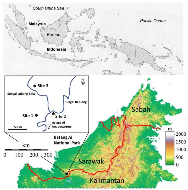
Figure 2.
Acoustic index time series. A series of acoustic complexity (ACI) and bioacoustic (BI) indices for each location. Columns represent traces from the same forest location, whereas the top row indicates traces of the ACIf and the bottom row is the BI for each 1-min recording. Dark- and light-shaded regions represent hours of darkness and daylight, respectively.
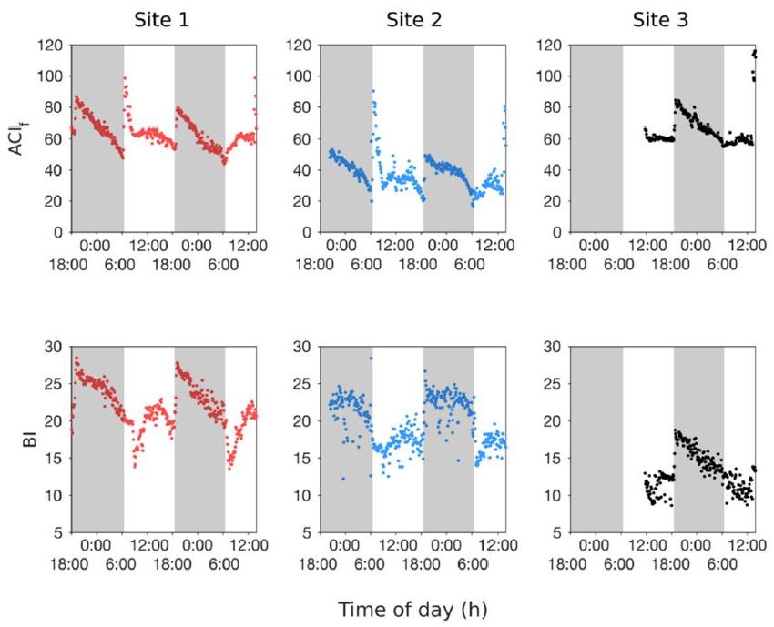
Figure 3.
Rainfall noise analysis. The three panels show the rainfall intensity index (RII) at each site for the duration of recording. The dashed lines in each panel indicate the threshold of the RII value (see Methods). The day–night cycle is represented by the shading. Times with suprathreshold RIIs are colored blue, whereas subthreshold values are grey. Note that at Site 1 and Site 2, there was a significant rainfall event on 02/22 around 6:00 h), and at all three recording sites there was another rainfall event near the end of the survey.
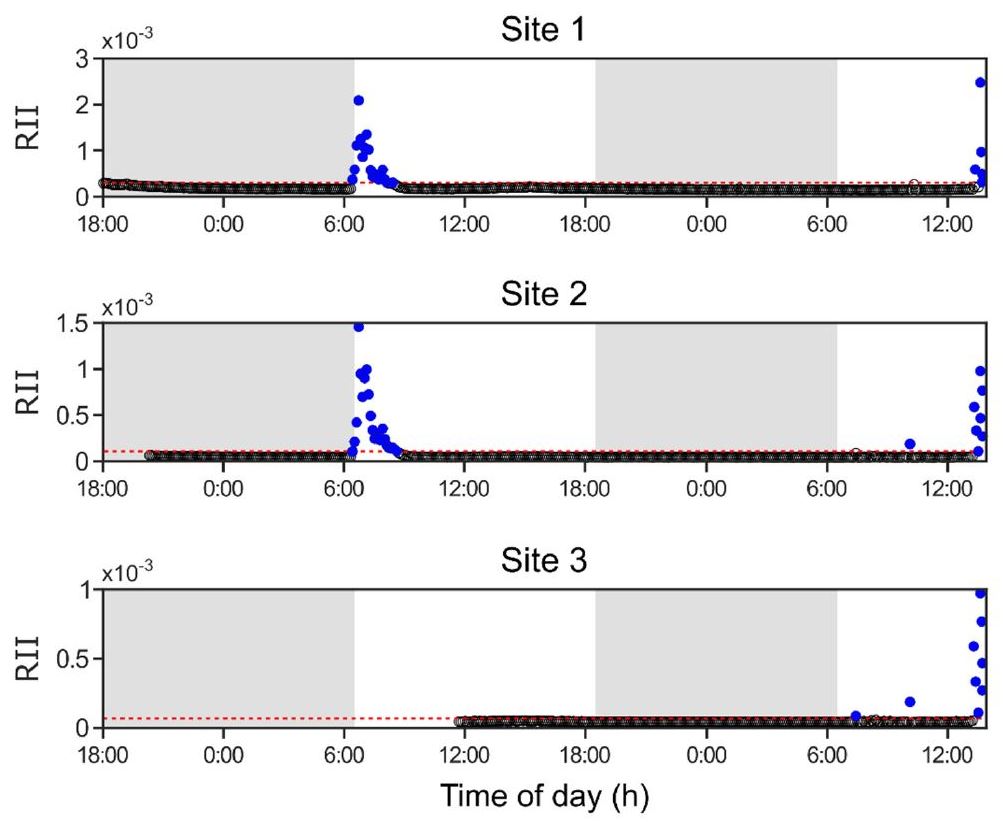
Figure 4.
Periodicity of acoustic indices. Spectra of (a) acoustic complexity (ACIf) and (b) bioacoustic (BI) indices for Site 1 are shown. The amplitudes were calculated using a Fast Fourier Transform (FFT) of the acoustic index time series for recordings taken at this site. The dashed lines indicate the upper 95th-percentile amplitudes calculated with an empirical bootstrap test (see Methods, Spectral Analysis). The autocorrelations for the (c) ACIf and (d) BI time series are also shown. Values were rescaled to fall between −1 and 1, representing the strength and sign of the correlation between the time series and a temporally shifted version. In both (a,b) and (c,d), prominent peaks exist at approximately 12 and 24 h, consistent with daily and twice-daily oscillations in the values of the acoustic index time series. Red curves represent ACIf measurements whereas blue curves indicate those for BI.
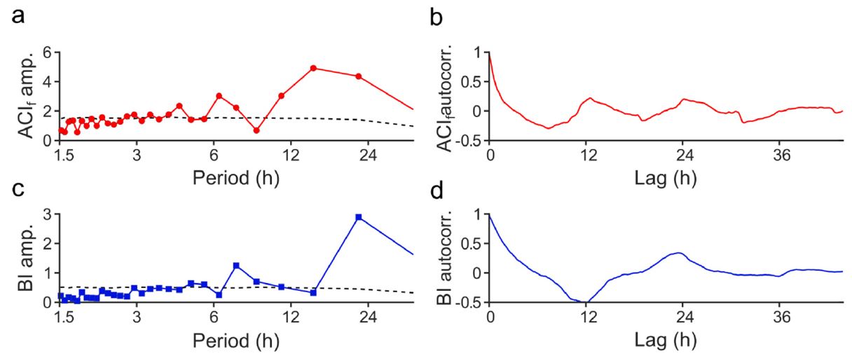
Figure 5.
Species richness time series. The avian and anuran species richness were quantified throughout the survey. Of note is the cyclical alternation of avian and anuran vocal activity which is phase-locked to the day-night transitions. The day-night cycle is represented by the shading.
Figure 5.
Species richness time series. The avian and anuran species richness were quantified throughout the survey. Of note is the cyclical alternation of avian and anuran vocal activity which is phase-locked to the day-night transitions. The day-night cycle is represented by the shading.
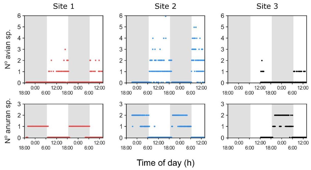
Figure 6.
Anuran call count. The frequency of individual frog vocalizations from species L. juliandringi (green) and L. parva (blue) was quantified as a function of time. The day–night cycle is represented by the shading.
Figure 6.
Anuran call count. The frequency of individual frog vocalizations from species L. juliandringi (green) and L. parva (blue) was quantified as a function of time. The day–night cycle is represented by the shading.
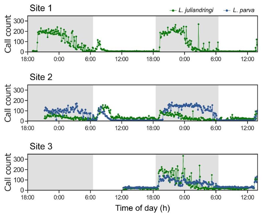

Table 1.
Correlation analysis. For the three recording sites, Spearman’s correlation values were calculated between the ACIf and BI with respect to five variables. In general, the correlations were the strongest between the variables corresponding to L. juliandringi and L. parva call rates and anuran species richness.
| Site 1 | Site 2 | Site 3 | ||||
|---|---|---|---|---|---|---|
| ACI | BI | ACI | BI | ACI | BI | |
| RII | 0.60 | 0.20 | 0.35 | −0.27 | 0.01 | −0.22 |
| Anuran richness | 0.30 | 0.81 | 0.57 | 0.77 | 0.75 | 0.84 |
| Avian richness | 0.25 | 0.18 | −0.32 | −0.47 | 0.24 | 0.21 |
| L. juliandringi calls | 0.81 | 0.79 | 0.75 | 0.33 | 0.86 | 0.86 |
| L. parva calls | — | — | 0.24 | 0.33 | 0.81 | 0.82 |
Table 2.
Information theory analysis. The value of the pairwise mutual information (MI, in units of bits) was calculated between the discretized ACIf and BI with respect to the discretized values of six variables (see Methods, Acoustic Index Correlations and Information Theory Analysis). It can be seen that the MI between the ACIf and BI with respect to the L. juliandringi and L. parva call rates was of higher strength (>0.7 bits) particularly for Site 1 and Site 3, whereas all other MI relationships were of lower strength. The MI value in brackets was not statistically significant. All other MI values were significant (p < 0.01).
| Site 1 | Site 2 | Site 3 | ||||
|---|---|---|---|---|---|---|
| ACI | BI | ACI | BI | ACI | BI | |
| RII | 0.12 | 0.06 | 0.18 | 0.07 | 0.15 | [0.01] |
| Day/night | 0.12 | 0.45 | 0.23 | 0.58 | 0.28 | 0.64 |
| Anuran richness | 0.12 | 0.50 | 0.35 | 0.57 | 0.32 | 0.69 |
| Avian richness | 0.03 | 0.09 | 0.22 | 0.46 | 0.04 | 0.09 |
| L. juliandringi calls | 0.83 | 0.65 | 0.55 | 0.14 | 0.93 | 0.85 |
| L. parva calls | — | — | 0.39 | 0.19 | 0.71 | 0.80 |
© 2021 Copyright by the authors. Licensed as an open access article using a CC BY 4.0 license.