An Ecoacoustic Snapshot of a Subarctic Coastal Wilderness: Aialik Bay, Alaska 2019

J_Ecoacoust 2020, 4(1), 2; doi:10.35995/jea4010002

Article

Timothy C Mullet

Kenai Fjords National Park, U.S. National Park Service, P.O. Box 1727, Seward, Alaska, U.S.A.; timothy_mullet@nps.gov

How to cite: Mullet, T.C. An Ecoacoustic Snapshot of a Subarctic Coastal Wilderness: Aialik Bay, Alaska 2019. J. Ecoacoust. 2020, 4(1), 2; doi:10.35995/jea4010002.

Received: 31 July 2020 / Accepted: 11 October 2020 / Published: 30 November 2020

Abstract

I recorded the ambient sounds at three locations in the wilderness of Aialik Bay in Kenai Fjords National Park, Alaska between 25 June and 21 September 2019. My aim was to capture an ecoacoustic snapshot of the coastal soundscape to provide a comparable baseline for evaluating wilderness characteristics defined by the Wilderness Act of 1964. I visually and empirically characterized the Aialik Bay wilderness soundscape using the acoustic metrics of soundscape power (normalized watts/kHz) and Normalized Difference Soundscape Index (NDSI) from 5373 five-minute recordings, combined with visual and aural spectral examination of 4386 recordings. Soundscape power exhibited similar patterns across frequency intervals with sound sources primarily occurring in the low-frequency (1–2 kHz) and mid-frequency (2–5 kHz) intervals. Significant differences within frequency intervals between sites suggested the presence of distinct sonotopes. Low-frequency sounds were dominant across all three sites with peak soundscape power values across study days and 24 h timeframes attributed to wind and occasional periods of technophony emitted from commercial tour boats and private boating activities. Low-frequency geophony from wave action was ever present. Technophony exhibited some predictable patterns consistent with the timing of sightseeing boat tours. Peak values of soundscape power at mid-frequencies were attributed to the geophony of rain. Although biophonies were less common than geophonies, the choruses of songbirds were prevalent in July and promptly occurred daily between 0300 and 0600. Biophonies generally declined over the course of the day. All sites displayed negative NDSI values over most study days and consistently negative values over 24 h time frames, indicating a soundscape primarily influenced by low-frequency geophony and periods of technophony. However, NDSI values showed patterns and peaks similar to biophonies at mid-frequency intervals indicating biophony was still a notable contribution to this geophony-dominant soundscape. Despite the acoustic footprint of motorboat noise detected at all sample sites, the soundscape of the Aialik Bay wilderness was dominated by the natural sounds of geophony, biophony, and occasional periods of natural quiet indicative of a wilderness only partially impacted by technophony.

Keywords:

Alaska; acoustic index; coastal; ecoacoustics; soundscape; wilderness

Introduction

The considerable loss of biodiversity over the last 100 years, compounded with climate change, underlines a significant shift in ecological processes and dramatic landscape change (Walther et al., 2002; Karl and Trenberth, 2003; VanLooy et al., 2006; Soja et al., 2007; Berg et al., 2009). Conservation land reserves, like those of the U.S. National Park Service (NPS), were set aside with the intention of being protected from human encroachment and to be preserved unimpaired for present and future generations to enjoy (Organic Act 1916). Unfortunately, national parks are suffering from environmental impacts caused by a variety of human activities in the wake of a rapidly developing society (Cole, 2012; Hansen et al., 2014). These impacts not only come at a cost to the ecological resources valued for preservation, but they also affect the enjoyment of humans who flock to these seemingly wild and pristine landscapes (Buckley and Foushee, 2012).

In the midst of all this change, Alaska is on the forefront of climate change-related impacts (Hinzman et al., 2005; Klein et al., 2005; VanLooy et al., 2006; Berg et al., 2009; Hess et al., 2019). The national parks of Alaska protect some of North America’s last undeveloped landscapes. Alaska’s national parks, therefore, present unique opportunities to experience the wild in the process of these changes. As such, visitors are enticed more now than ever to see how Alaska’s national park landscapes are changing with visitations having increased from 1 million visitors/year in 2005 to 2.9 million in 2018 (Christian, 2019). This increase in visitation also brings with it an increase in motorized activities.

Preserving these wild landscapes in perpetuity for their ecological integrity and human benefit marks a significant challenge for park management as the inadvertent impacts of human activity degrade wilderness quality (Cole, 2012). Wilderness in national parks is an anthropocentrically defined resource that involves the identification of administrative boundaries where wilderness qualities exist in the landscape (Wilderness Act 1964). The Wilderness Act defines the characteristics of wilderness as an area (1) “where the earth and its community of life are untrammeled by man,” (2) “of undeveloped Federal land retaining its primeval character and influence,” (3) that “generally appears to have been affected primarily by the forces of nature,” and (4) that provides “outstanding opportunities for solitude.”

Landscapes that uphold these definitions can be officially designated as wilderness units by the U.S. Congress, hereafter referred to as Congressionally designated Wilderness (CW). Congressional designation enables the legislation of the Wilderness Act with mandates that define CW boundaries and guidance to preserving its character (Wilderness Act 1964). Landscapes within federal land reserves that retain the definitions of wilderness character but have not yet been designated by Congress are considered eligible wilderness (EW). Collectively, CW and EW are hereafter referred to as Wilderness. Roughly 95% of the NPS in Alaska has some level of Wilderness protection. It is the definition of Wilderness character that challenges land managers with preserving its quality as climate change and the proliferation of mechanized transports continue to alter its landscapes (Cole, 2012; Mullet et al., 2017a).

Establishing a snapshot in time of the current status of Wilderness is imperative to assess the natural processes of succession in a changing climate and the potential impacts of mechanized activities on Wilderness character. However, it may also be beneficial to visitors seeking to gain a better understanding and appreciation of Wilderness in a changing world through education. Perhaps more importantly, establishing a baseline snapshot in time of Wilderness characteristics can provide a foundation of reference on how or whether these landscapes retain their eligibility under the definitions of the Wilderness Act. As human activity and climate change continue to influence the landscape, evaluation of Wilderness characteristics may move management into a more active role to preserve its quality (Cole, 2012).

Sound is an inherent component of Wilderness (Mullet et al., 2017a), playing an important role in ecological processes (Farina and Gage, 2017) and influencing the emotional states of human beings (Moscoso et al., 2018) and their perceptions of environmental quality (Carles et al., 1999; Traux, 2001; Romero et al., 2015). However, soundscapes as a whole and their components of biophony, geophony, and technophony are not simply an attribute of Wilderness but also indicators of Wilderness quality (Mullet et al., 2017a). Where natural activities of soniferous species and geophysical events dominate the landscape, biophony and geophony are evident, signifying an intact Wilderness characterized by naturalness. Naturalness also includes the sustained integrity of ecological systems where natural processes sustain acoustic habitats (Mullet et al., 2017b) for a variety of acoustic communities (Farina and James, 2016) that have evolved in a pre-mechanized world. Contrarily, where human mechanization is present within or adjacent to Wilderness areas, technophony will also be present, indicating the diminished Wilderness characteristics of naturalness and solitude.

Ecoacoustics utilizes the measurable attributes of soundscapes to characterize the status of environmental quality, ecological integrity, and human’s perceptions of nature (Carles et al., 1999; Farina and Gage, 2017; Moscoso et al., 2018). These methodologies also extend these characterizations to future discoveries of how ecosystems change over time with the soundscape serving as the litmus of measurable detection (Krause et al., 2011; Krause and Farina, 2016). In this context, soundscapes may provide insights into the ecological changes that are occurring in Wilderness areas as a result of human activity and climate change.

Few peer-reviewed ecoacoustic studies have focused specifically on terrestrial subarctic regions of Alaska (Mullet et al., 2016, 2017a) or Alaskan Wilderness in particular (Miller et al., 2018; Mullet et al., 2017a). The NPS Natural Sounds Program has established baseline sound pressure levels at a variety of national parks, including Alaska (Lynch et al., 2011), and have explored a variety of ecoacoustic-related topics with reports, articles, teaching materials, and sound galleries available at https://www.nps.gov/subjects/sound/references.htm. Yet, there has not been a focus on characterizing ecological patterns represented by, and attributed to, soundscapes as a component of Wilderness character in Alaska. The myriad of sounds emitted in a Wilderness soundscape signifies the ecological patterns and processes that form the natural character of the Wilderness landscape (Pijanowski et al., 2011; Mullet et al., 2017a). These Wilderness soundscapes are psychologically interactive with human visitors through an individual’s sense of solitude which may also be negatively affected by the intrusion of technophony (Carles et al., 1999; Traux, 2001; Mace et al., 2004).

Capturing an ecoacoustic snapshot in time of a Wilderness soundscape can provide useful information about the current status of naturalness and solitude within Wilderness areas. Using soundscape metrics, these Wilderness characteristics can be quantified and measured against future soundscape data to evaluate the potential trends in Wilderness degradation or the altered state of Wilderness eligibility in a changing environment. My objective was to characterize the spatio-temporal variation of a Wilderness soundscape in an Alaskan national park with a focus on the patterns of biophony, geophony, and technophony over the summer season when human visitation primarily occurs.

Methods

Study Area

I conducted my research in Kenai Fjords National Park (KEFJ) located on the eastern Kenai Peninsula of south-central Alaska (Figure 1). Kenai Fjords National Park includes 2000 km² of the Harding Icefield from which dozens of glaciers extend into the Gulf of Alaska carving out steep fjord systems with approximately 700 km² of varying successional stages of coastal maritime rainforest. This dynamic ecoregion consists of a diverse array of ecosystems that include intertidal communities, coastal meadows, anadromous riparian systems, subalpine shrublands, mixed conifer-deciduous forests, old growth mountain hemlock (Tsuga martensiana) forests, and alpine tundra. Elevations range from sea level to 1970 m and temperatures can range from −30 to 4 °C in winter (November–April) and 10 to 25 °C in summer (June–August) (PEDA2 RAWS data Alaska; https://mesowest.utah.edu/). Average annual precipitation has ranged from 18.3–38.3 cm between 2012 and 2019 with annual snow depth averaging 8.7–89.1 cm over the same period (PEDA2 RAWS data Alaska; https://mesowest.utah.edu/).

Kenai Fjords National Park manages 2304 km² of its jurisdictional land as EW. The variety of ecosystems encompassed by KEFJ EW provides an outstanding and diverse sonic environment generated by geophysical processes and soniferous animal communities and mechanized human transports. I focused my study efforts in the highly visited coastal wilderness of Aialik Bay, a region that is only accessible by boat, plane, or helicopter (Figure 1). Aialik Bay possesses two tidewater glaciers (Aialik and Holgate) and one lake-terminating glacier (Pedersen) that are popular sightseeing locations for boat and air tours. This glacially influenced fjord system is dominated by conifer forests, subalpine shrub, and alpine tundra with an array of freshwater streams and lakes fed by snow melt from the surrounding glaciers and mountain peaks, supporting a variety of wildlife.

Site Selection

Three sample sites were selected so that all had the acoustic vantage point of capturing marine- and terrestrial-based sound sources (Figure 1). Each site provided a different spatial coverage of the fjord and represented three different habitat types at varying elevations and distances to the coast (Table 1). These sites included Aialik Bay Ranger Station (ABRS), Holgate Public Use Cabin (HOLG), and McMullen Cove (MCML) (Figure 1). All sample sites were generally located within forested edge habitats to the coast.

Acoustic Sampling

SM4 Song Meters (Wildlife Acoustics, Inc., Maynard, MA, USA) were used to record the acoustic environment in right-channel, mono-aural, at a sample rate of 22,050 Hz for a useable frequency up to 11,000 Hz. Recordings were conducted for five minutes every 55 min for a total of 120 min of acoustic recordings per day. Microphones were calibrated to the default sound pressure level of 94 dB. Sound recorders were mounted to the trunks of trees at approximately two meters above the ground. Microphones were omnidirectional and were mounted to prevent obstruction from all sides. The standard stock foam microphone covers were used to reduce wind disturbance to the microphone’s surface. Sound data were saved to 32 GB SD cards in WAV format and archived in KEFJ’s sound database. Sound monitoring was initiated at ABRS on 25 June 2019 and at HOLG and at MCML on 27 June 2019. Sound recorders were visited in July and August for maintenance and data collection then retrieved on 21 September 2019.

Sound events were captured for the entire duration of the sampling period at HOLG and MCML from 27 June to 21 September 2019 totaling 86 study days. This equated to 2065 and 2060 five-minute sound recordings, respectively. Acoustic sampling at ABRS was reduced to 35 study days and 1248 recordings from 25–26 June, 07–26 July, and 20 August–21 September 2019 due to bears tampering with and dismantling equipment.

Acoustic Measures

While a variety of acoustic metrics and indices are available (Bradfer-Lawrence et al., 2019), the intention of this study was to utilize the figurative “lens” of soundscape power (Kasten et al., 2012) and NDSI (Gage and Axel, 2014) to describe the current state of the Aialik Bay coastal wilderness. Soundscape power has been successfully used to describe soundscapes in south-central Alaska (Mullet et al., 2016, 2017a) and coastal soundscapes in the Pacific Northwest (Ritts et al., 2016). Although NDSI has not yet been applied to subarctic ecosystems, NDSI is based on the metric of soundscape power (normalized watts/kHz) so it was expected that NDSI could be a useful descriptor as it has been in other studies (Gage and Axel, 2014; Fuller et al., 2015; Eldridge et al., 2016; Schindler et al., 2020).

Acoustic measures were computed in R statistical environment (R Core Team, 2014) using the soundecology (Villanueva-Rivera and Pijanowski, 2013) and seewave-R (Sueur et al., 2008) packages. Computations derived soundscape power after Kasten et al. (2012) as the normalized power spectral density (watts/kHz) at 1 kHz frequency intervals for the frequency ranges of 1000–11,000 Hz for each five-minute sound recording. The NDSI was calculated as the ratio of soundscape power (normalized watts/kHz) corresponding to frequency intervals commonly associated with technophony (1–2 kHz) and biophony (>2 kHz) as described by Gage and Axel (2014).

NDSI = \frac{(B i o p h o n y - T e c h n o p h o n y)}{(B i o p h o n y + T e c h n o p h o n y)}

(1)

Data and Spectral Analysis

Figures and statistical analyses were done in Minitab^® 19.1.1 (Minitab, LLC. 2019). The patterns of soundscape metrics (i.e., soundscape power, NDSI) were visualized and described for each sample site over frequency intervals, study day, and 24 h timeframes. Statistical differences in soundscape power and acoustic indices were compared between sample sites, across study days, and across 24 h timeframes using 95% confidence intervals (CI). A Pearson’s correlation was calculated to determine the relationship between low frequencies (1–2 kHz) and mid-frequencies (2–5 kHz) where soundscape power was concentrated.

Aural and visual spectral analysis was conducted in Audacity^® 2.2.2 (https://www.audacityteam.org/) for 4386 sound recordings associated with distinct peak and minimum soundscape power values over study days. Peak values of soundscape power were defined at the 1–2 and 2–5 kHz intervals on study days with mean values >0.95 normalized watts/kHz and >0.3 normalized watts/kHz, respectively. Minimum values for the 1–2 and 2–5 kHz intervals were identified on study days displaying mean soundscape power values <0.6 normalized watts/kHz and <0.1 normalized watts/kHz, respectively. Each five-minute sound recording was visually inspected as a spectrogram to identify spectral signatures representing unique sound sources. Recordings were then aurally inspected in order to identify specific sound sources associated with study days (Figure 2).

Results

Soundscape Power by Frequency Interval and Site

The pattern of soundscape power over 11 1 kHz frequency intervals (1–11 kHz) was similar across all sample sites (Figure 3). Soundscape power was highest for the 1–2 kHz frequency interval than all other intervals followed by a drop in soundscape power at the 2–3 kHz frequency interval. Soundscape power steadily declined for all subsequent frequencies with the 10–11 kHz interval having the lowest value overall. There was no single frequency interval where the values of soundscape power were similar across all three sample sites (Figure 3). ABRS displayed higher soundscape power than HOLG and MCML between 2–4 kHz and lower values than both sites between 7–11 kHz. HOLG exhibited higher soundscape power than ABRS and MCML between 4–7 kHz and similar values to MCML between 7–9 kHz. MCML had the highest soundscape power values than ABRS and HOLG within the 1–2 and 9–11 kHz frequency ranges (Figure 3).

Temporal Variation of Soundscape Power

Soundscape power was variable across study days and 24 h timeframes, exhibiting peak and minimum values for particular days and hours over each sample site and frequency interval. However, 95% CI intervals revealed numerous days of overlap across study days and more substantial overlap over hourly intervals. Soundscape power at the 1–2 and 2–5 kHz intervals showed distinct patterns of fluctuating values over study days and 24 h timeframes with spectral analysis revealing specific ecoacoustic events contributing to data extremes. Soundscape power at frequencies of 5–11 kHz exhibited significantly lower values of soundscape power than all other frequency intervals with spectral analysis revealing sounds generated by rare instances of high-frequency (5–11 kHz) biophony from songbirds and intermittent geophony associated with rain.

I consequently focused analyses on the soundscape power at the 1–2 kHz intervals and averaged the soundscape power across the 2–5 kHz frequency intervals as representative of the Aialik Bay EW soundscape. Patterns of soundscape power across the entire 86 days at HOLG and MCML were comparable to the temporal patterns in soundscape power of ABRS despite gaps in the ABRS data set. Soundscape power at the 1–2 kHz frequency interval was consistently inversely correlated to that of the 2–5 kHz interval for all sample sites over time (Pearson’s R: ABRS = −0.905 [p < 0.0001]; HOLG = −0.815 [p < 0.0001]; MCML = −0.811 [p < 0.0001]).

Temporal Variation of Low-Frequency Sounds by Study Day

Study days with peak values within the 1–2 kHz interval (>0.95 normalized watts/kHz) included 11 days at ABRS, 12 days at HOLG, and 21 days at MCML (Figure 4). All sites exhibited similar peak values on 16 July 2019 and 23 August 2019. Peak values of soundscape power were also similar at HOLG and MCML on 04 September 2019 (Figure 4). Boat noise, waves, and wind were the primary sound sources contributing to peak values on 16 July and 23 August 2019 while boat noise and wind were the two sound sources contributing to peak soundscape power values on 04 September 2019. Overall, wind was the highest proportional (51%) sound source to all study days with peak values followed by waves (39%), boat noise (7%), bees (2%), and rain (1%) (Figure 5).

Study days with minimum soundscape power values within the 1–2 kHz interval (<0.6 normalized watts/kHz) included 12 days at ABRS, eight days at HOLG, and one day at MCML (Figure 4). All sample sites had similarly low values on 14 July 2019 while ABRS and HOLG had similarly low values on 07 July and 01–02 September 2019 (Figure 4). Rain and wind were the dominant sound sources within the 1–2 frequency interval on 14 July 2019. Wind and waves were the primary sound sources at ABRS and HOLG on 07 July 2019. Wind and rain were the dominant sound sources at ABRS and HOLG on 01 and 02 September 2019.

Geophony from wind was proportionally higher (56%) than all other sound sources on study days with the lowest soundscape power (Figure 5). Geophony from rain (26%), waves (14%), and technophony from boat noise (3%) and airplane noise (1%) contributed the remaining proportion of sound sources (Figure 5). Wind events were more subtle on days with low soundscape power than days with peak soundscape power when wind events were more intense. Heavy rain associated with mid- and high frequencies was a prominent acoustic event during study days of low soundscape power values.

Temporal Variation of Mid-Frequency Sounds by Study Day

Study days with peak values of soundscape power within the 2–5 kHz interval (>0.3 normalized watts/kHz) by study day included 13 days at ABRS, 12 days at HOLG, and five days at MCML (Figure 6). Inverse to the lowest soundscape power values within the 1–2 kHz interval, peak values of soundscape power within the 2–5 kHz interval were recorded at all sample sites on 14 July and 1 September 2019 (Figure 6). Peak values were similar at ABRS and HOLG on 7 July, 31 August, and 2 September 2019 (Figure 6). Peak soundscape power values were also similar for ABRS and MCML on 07 and 12 September 2019 (Figure 6). Soundscape power also exhibited similar peak values at HOLG and MCML on 27 July 2019 (Figure 6).

Wind, songbird choruses, and rain were the most common sound sources on 14 July 2019 while wind, rain, and the calls of seabirds were the prominent sound sources on 1 September 2019 at all sample sites. Seabird calls, waves, and rain were the primary sound sources shared at ABRS and HOLG on 7 July, 31 August, and 2 September 2019. Wind and rain were the sole sound sources at ABRS and MCML on 7 and 12 September 2019 while rain was the most common sound source shared between HOLG and MCML on 27 July.

Biophonies from songbirds and geophonies from rain and waves were the most common sound sources contributing to peaks in soundscape power within the 2–5 kHz interval during July. Aural and visual spectral analyses revealed that there was a general decline in biophonies from July to August with occasional calls of individuals in September rather than choruses. Heavy rains in September filled the acoustic space that had previously been occupied by biophonies earlier in the season. Geophony from rain was proportionally the greatest contributing sound source (46%) to study days with peak soundscape power values within the 2–5 kHz interval (Figure 7). However, biophony from songbirds was still a notable proportion (29%) of mid-frequency sound sources (Figure 7). Geophonies from waves (15%) and wind (7%) and biophonies from seabird calls (3%) made up the remaining proportion of sound sources (Figure 7).

Study days with the lowest values of soundscape power within the 2–5 kHz interval (<0.1 normalized watts/kHz) included 12 days at ABRS, nine days at HOLG, and one day at MCML (Figure 6). All three sites displayed similarly low values on 16 July 2019 and ABRS and HOLG displayed similarly low values on 15 July 2019 (Figure 6). Geophony from rain and wind and biophony from songbirds were the most common sound sources on 15 and 16 July 2019. Geophony from wind contributed 60% to study days with the lowest soundscape power followed by sounds from waves (15%), songbird choruses (11%), rain (8%), and seabird calls (7%) (Figure 7).

Study days dominated by wind were generally low in sound energy and absent of biophony, technophony, and intense geophonic events (e.g., high winds, rain) which created a subtle quiet acoustic environment. These natural quiet events occurred at all sample sites but displayed no discernable pattern by study day. Sound recorders captured rain events in mid-July and early and mid-September. Songbird choruses would occasionally cooccur with light rain events, but full choruses primarily took place in the absence of other sound sources and occurred most regularly between 29 June to 16 July 2019 after which time songbird choruses were reduced to the calls of individuals in August and September.

Temporal Variation of Low-Frequency Sound by Time of Day

Low-frequency soundscape power at ABRS indicated higher values in the evening hours between 2200–0200 when the acoustic space was dominated by the geophonies of rain and wind (Figure 8). A distinct decline in low-frequency soundscape power occurred at 0300–0400 when wind and rain events subsided (Figure 8). Moderate increases between 0500–1400 were primarily geophonies of wind and rain events with peaks in occurrence of technophony from boat noise between 1200 and 1400 (Figure 8). Boat noise was the dominant sound source between 1600 and 1800 interspersed with periods of rain and wind between 1500 and 2100 (Figure 8).

Low-frequency soundscape power at HOLG was highest between 2200 and 0200 during periods of intense rain, wind, and wave activity (Figure 8). Soundscape power decreased between 0200 and 0300 but was followed by small fluctuations in soundscape power between 0400 and 1100 that was primarily attributable to rain, wind, and wave activity between 0500 and 1100, interspersed with boat noise between 0900 and 1100 (Figure 8). This diurnal period gave way to a gradual increase in soundscape power between 1200 and 1600 generated by an increase in boat noise from 1200–1400 cooccurring with periods of rain, wind, and wave activity from 1200–1600 (Figure 8). Soundscape power generated by boat noise, rain, wind, and wave activity declined from 1700–2100 before rising to peak values of geophonic events in the evening (Figure 8).

Low-frequency soundscape power at MCML was highest between 2000 and 0200 during periods of rain, wind, and wave activity (Figure 8). Fluctuations in soundscape power at MCML between 0300 and 1900 were largely attributed to fluctuations in rain, wind, and wave activity (Figure 8). Occasional periods of boat noise were documented during the hours of 0800 and 1400 (Figure 8).

Temporal Variation of Mid-Frequency Sound by Time of Day

Mid-frequency soundscape power at ABRS was lowest during the hours between 2200 and 0200 with the periodic calls of songbirds and seabirds and intermittent rain (Figure 9). Peak periods of soundscape power were between 0300 and 1100 and 1800–2100 where biophonies from songbird choruses and geophony from rain were common (Figure 9). Mid-frequency soundscape power at HOLG exhibited similar patterns over 24 h timeframes as ABRS (Figure 9). The lowest values at HOLG occurred during 2200–0100 when intermittent songbird calls were present along with the geophonies of waves and rain (Figure 9). The highest soundscape power values at HOLG occurred during 0300–0500 and 1200–1800 when a mix of songbird choruses, seabird calls, rain, wind, and waves occurred (Figure 9). Mid-frequency soundscape at MCML displayed four distinct peaks at 0400, 0700, 1300, and 1900 (Figure 9). Songbird choruses, rain, and waves were the sound sources at 0400 while rain and wind were attributed to 0700, 1300, and 1900. The lowest soundscape power values occurred during 2200–0200 when mid-frequency intervals were occupied by the geophonies of rain, wind, and waves (Figure 9).

Temporal Variation of NDSI

Temporal patterns in NDSI varied by sample site, study day, and over 24 h timeframes. Values of NDSI were negative for all sample sites with values sequentially lower at ABRS (Mean = −0.113 [95% CI = −0.141, −0.085), HOLG (Mean = −0.153 [95% CI = −0.170, −0.135], and MCML (Mean = −0.229 [95% CI = −0.242, −0.216]). The NDSI values across study days mirrored the temporal patterns of soundscape power values of the 2–5 kHz frequency interval over the same period with only five days significantly deviating between metrics (Figure 6 and Figure 10). However, positive NDSI values were only present on 10 study days at ABRS, five study days at HOLG, and zero study days at MCML (Figure 10). Study days with positive NDSI values were attributed to the geophony from mid-frequency rain. Negative NDSI values represented the dominance of low-frequency geophonies from waves and wind relative to the presence of mid- and high-frequency biophonies and geophonies (Figure 10).

The patterns of mean NDSI values over 24 h timeframes were all negative for each sample site (Figure 10). Peak NDSI values were evident at ABRS and HOLG between 0300 and 0400 (Figure 10). These peaks were consistent with the early morning rise in soundscape power values within the 2–5 kHz frequency interval representative of the dawn chorus (Figure 9). The values of NDSI at MCML exhibited a more regular pattern with no significant fluctuations (Figure 10). These results were largely attributed to the regularity in geophony associated with wave action.

Discussion

The wilderness soundscape of Aialik Bay in Kenai Fjords National Park, over the summer of 2019, consisted of distinct patterns of biophony, geophony, and technophony across space that coincided with the processes of geophysical, biological, and anthropogenic phenomena over time. The distribution of soundscape power over frequencies had similar patterns across all sample sites. Much like what was observed of coastal soundscapes in British Columbia, Canada (Ritts et al., 2016), low-frequency geophony presented the most dominant acoustic component in the overall coastal EW soundscape in Aialik Bay. However, soundscape power was not homogenous between sample sites suggesting the presence of distinct sonotopes (Farina, 2014).

All sample sites had the occurrence of boat-generated technophony. Yet, HOLG and MCML had proportionally more technophony from boats than ABRS. Boat noise was consistently present at specific times of the day at HOLG between 1200 and 1400. These ecoacoustic events coincided with daily scheduled tour boat activities traveling to and from Holgate Glacier. Boat-generated technophony at MCML was largely associated with smaller motors likely generated from private recreation vessels occurring at unpredictable time periods throughout the day. Technophony at ABRS was largely a combination of noise emitted from small, private vessels and larger, commercial tour boats.

Biophonies generated by songbird communities were proportionally higher at ABRS than all other sample sites with HOLG having the second highest proportion of biophony generated by songbird communities. Other sources of biophony were the calls of seabirds and the buzzing of bees. Seabird calls were proportionally higher at ABRS than HOLG but not documented at MCML. It is not clear why seabird calls were more common at ABRS than HOLG and not present at MCML. Conversely, the low-frequency buzzing of bees was only recorded at MCML likely due to the recorder being inadvertently placed near a hive.

The temporal patterns of mid-frequency biophony were associated with distinct peaks on study days when technophony and/or geophony (i.e., wind) were low. Many studies have found this same strong negative relationship between the occurrence of biophony and the low-frequency sounds of geophony and technophony (see Farina, 2017 for a review). This inverse relationship in Aialik Bay may be due to the impacts that environmental noise has on biophonies (Brumm, 2004) and the physical effects these wind and rain events can have on animal behavior.

Biophonies from songbird choruses were the greatest contributor to peak soundscape power values at mid-frequencies in July at ABRS and HOLG, but not at MCML. The prevalence of songbird choruses declined at the end of July when only individual calls contributed to biophony in August and September. Geophonies from rain events became the most prevalent sound source of peaks in mid-frequency soundscape power in August and September. Patterns in mid-frequency soundscape power at the 24 h timeframe were specifically associated with the biophonies of songbird choruses. Data revealed that songbird choruses began daily in July around 0300 and maintained a moderate fluctuation and decline in soundscape power and soniferous activity throughout the day until 2200 after which bird choruses would cease.

Although a dawn chorus was evident, there was no clear pattern in soundscape power that distinguished a dusk chorus typical of lower latitude temperate environments (Malavasi and Farina, 2012). Due to long periods of daylight that are available in June and July in south-central Alaska and the lack of nocturnal soniferous organisms vocalizing below 11,000 Hz, biophony was largely sustained by songbird choruses and remained so for up to 19 h of the day at its peak. A distinct decline and eventual absence of bird songs in August and September was evidence of the short breeding period many species experience in the subarctic (Eeva et al., 2000). These data can be useful for future comparisons in biophonic activity as climate change continues to influence the phenology of some songbirds (Both and te Marvelde, 2007; Gordo, 2007; Charmantier and Gienapp, 2014).

Like the acoustic footprint of snowmobile noise in CW areas of the western Kenai Peninsula (Mullet et al., 2017a), technophony from boat noise extended into the terrestrial region of Aialik Bay’s EW well beyond the marine location from which it came. This included the ABRS sample site located 86.2 m from the coastline. Although a specific measurable technophonic effect on biophony was not apparent in the data, the occurrence of technophony during the afternoon and early evening hours of the day were synchronous with time periods when park visitors are actively experiencing the Aialik Bay EW. The highest levels of technophony associated with boat noise occurred at HOLG where a cabin is located for visitors seeking to experience solitude in this wilderness setting. Even though airplane and motorboat noise had a much lower proportion of occurrence than natural sounds, this form of technophony is likely audible throughout many coastal locations in Aialik Bay’s EW at a variety of intensities.

Natural soundscapes are known to have important value to tourists’ experience (Romero et al., 2015; Liu et al., 2017; Ren et al., 2018). Yet, given that KEFJ is visited by a diversity of people from all over the world, the array of values individuals assign to technophony in wilderness (Nash, 2014) and soundscapes in park settings (Jiang et al., 2017; Ren et al., 2018) may require management to evaluate the impact technophony could have on the fundamental definitions of Wilderness naturalness and solitude. The international appeal of KEFJ makes these cultural differences an added component to EW evaluation.

Ironically, nearly all human experiences in KEFJ EW are facilitated by boats. This highlights the conundrum of Alaska’s public lands where the preservation of Wilderness character, free from mechanization, is challenged by the means of providing humans access to Wilderness areas (Mullet et al., 2017a). Further complications for KEFJ Wilderness management arise in that the noise that degrades Wilderness character is completely derived from human activity outside its jurisdictional boundaries. With park visitations on the rise and plans to increase commercial tour boat and cruise ship operations in the region, the status of KEFJ’s Wilderness eligibility in Aialik Bay is uncertain. However, many other areas of KEFJ’s coastal fjords outside Aialik Bay may have different soundscape characteristics, requiring further study.

More notably, recordings did capture times at all sample sites when natural quiet conditions occurred over the study period. Despite technophony’s acoustic footprint on these three locations, the presence of natural quiet when technophony and biophony were absent and geophony was at its lowest energy, the quiet solitude of Aialik Bay’s EW was still present. This was also a characteristic of the winter soundscape in the CW within the adjacent Kenai National Wildlife Refuge (Mullet et al., 2017a) indicating Wilderness areas on the Kenai Peninsula encompass an assortment of geophysical, biological, and anthropogenic phenomena that present complex patterns and processes in the landscape.

Conclusion

The results of this study reflect four important ecoacoustic characteristics of the Aialik Bay EW soundscape: (1) Geophony from wind, waves, and rain is a significant contributor to this coastal soundscape; (2) Technophony from boats has a periodic acoustic footprint that can likely extend >100 m into the terrestrial landscape with degrading effects to naturalness and solitude; (3) Biophony from bird choruses is higher in activity across daily periods between July and August and 24 h periods between 0300 and 0600; and (4) Naturalness and solitude attributed to natural ecoacoustic processes of geophony and biophony currently dominate the soundscape.

The status of KEFJ’s EW naturalness is already in the process of change. With the rapid changes of Aialk Bay’s glaciers, compounded with milder winters, warmer summers, changes in precipitation regimes, seabird die-offs, and fire becoming more common on the western side of the Peninsula, it is likely that the ecological patterns and processes of Aialik Bay’s landscape will be much different in the future than it is now (VanLooy et al., 2006; Hayward et al., 2017; Magness and Morton, 2018). This descriptive analysis of the Aialik Bay EW soundscape sets a baseline of information for future comparisons. Annual sampling of the area can conceivably reveal acute variations in soundscape components, documenting incremental change. Long-term sampling will provide a broader temporal view of whether the soundscape is changing with increased human activity (e.g., technophony) and climate change-related impacts to the biological and geophysical environment represented by biophony and geophony.

Funding

This research was funded by U.S. National Park Service.

Acknowledgments

This project was funded by the U.S. National Park Service. Field work was assisted by K. Mocnik and N. Bawtinhimer. Additional support was provided by the staff of Kenai Fjords National Park. I give a special thank you to A. Farina and two anonymous reviewers for their excellent editorial advice to improve this manuscript. This study is dedicated to the late Stuart H. Gage who inspired this work. The findings and conclusions in this article are those of the authors and do not necessarily represent the views of any government agencies. Any use of trade, product, or firm names is for descriptive purposes only and does not imply endorsement by the U.S. government.

Conflicts of Interest

The author declares no conflict of interest.

References

Berg, E. E.; Hillman, K. M.; Dial, R.; DeRuwe, A. Recent woody invasion of wetlands on the Kenai Peninsula Lowlands, south-central Alaska: A major regime shift after 18 000 years of wet Sphagnum–sedge peat recruitment. Canadian Journal of Forest Research 2009, 39(11), 2033–2046. [Google Scholar] [CrossRef]
Both, C.; te Marvelde, L. Climate change and timing of avian breeding and migration throughout Europe. Climate Research 2007, 35(1–2), 93–105. [Google Scholar] [CrossRef]
Bradfer-Lawrence, T.; Gardner, N.; Bunnefeld, L.; Bunnefeld, N.; Willis, S. G.; Dent, D. H. Guidelines for the use of acoustic indices in environmental research. Methods in Ecology and Evolution 2019, 10(10), 1796–1807. [Google Scholar] [CrossRef]
Brumm, H. The impact of environmental noise on song amplitude in a territorial bird. Journal of Animal Ecology 2004, 73(3), 434–440. [Google Scholar] [CrossRef]
Buckley, L. B.; Foushee, M. S. Footprints of climate change in US national park visitation. International Journal of Biometeorology 2012, 56(6), 1173–1177. [Google Scholar] [CrossRef] [PubMed]
Carles, J. L.; Barrio, I. L.; De Lucio, J. V. Sound influence on landscape values. Landscape and Urban Planning 1999, 43(4), 191–200. [Google Scholar] [CrossRef]
Charmantier, A.; Gienapp, P. Climate change and timing of avian breeding and migration: Evolutionary versus plastic changes. Evolutionary Applications 2014, 7(1), 15–28. [Google Scholar] [CrossRef]
Christian, P. National Park Service Visitation in Alaska Tops 2.9 Million in 2018; National Park Service, Region 11. Retrieved November 2, 2019; 15 March 2019; from https://www.nps.gov/orgs/1840/national-park-service-visitation-in-alaska-tops-2-9-million-in-2018.htm.
Cole, D. N. Beyond naturalness: Adapting wilderness stewardship to an era of rapid global change. International Journal of Wilderness 2012, 18(2), 9–14. [Google Scholar]
Eeva, T.; Veistola, S.; Lehikoinen, E. Timing of breeding in subarctic passerines in relation to food availability. Canadian Journal of Zoology 2000, 78(1), 67–78. [Google Scholar] [CrossRef]
Eldridge, A.; Casey, M.; Moscoso, P.; Peck, M. A new method for ecoacoustics? Toward the extraction and evaluation of ecologically-meaningful soundscape components using sparse coding methods. PeerJ 2016, 4, e2108. [Google Scholar] [CrossRef]
Farina, A.; Gage, S. H. (Eds.) Ecoacoustics: The ecological role of sounds; Wiley: New Jersey, 2017. [Google Scholar]
Farina, A. Soundscape Ecology: Principles, patterns, methods, and applications; Springer: Dordrecht, Netherlands, 2014. [Google Scholar]
Farina, A. The ecological effects of noise on species and communities. In Ecoacoustics. The ecological role of sounds; Farina, A., Gage, S. H., Eds.; Wiley: New Jersey, 2017; pp. 95–107. [Google Scholar]
Farina, A.; James, P. The acoustic communities: Definition, description, and ecological role. Biosystems 2016, 147, 11–20. [Google Scholar] [CrossRef]
Fuller, S.; Axel, A. C.; Tucker, D.; Gage, S. H. Connecting soundscape to landscape: Which acoustic index best describes landscape configuration? Ecological Indicators 2015, 58, 207–215. [Google Scholar] [CrossRef]
Gage, S. H.; Axel, A. C. Visualization of temporal change in soundscape power of a Michigan lake habitat over a 4-year period. Ecological Informatics 2014, 21, 100–109. [Google Scholar] [CrossRef]
Gordo, O. Why are bird migration dates shifting? A review of weather and climate effects on avian migratory phenology. Climate Research 2007, 35(1–2), 37–58. [Google Scholar] [CrossRef]
Hansen, A. J.; Piekielek, N.; Davis, C.; Haas, J.; Theobald, D. M.; Gross, J. E.; Monahan, W. B.; Olliff, T.; Running, S. W. Exposure of U.S. National Parks to land use and climate change 1900–2100. Ecological Applications 2014, 24(3), 484–502. [Google Scholar] [CrossRef]
Hayward, G. H.; Colt, S.; McTeague, M. L.; Hollingsworth, T. N. (Eds.) Climate change vulnerability assessment for the Chugach National Forest and the Kenai Peninsula; (General Technical Report PNW-GTR-950); U.S. Department of Agriculture, Forest Service, Pacific Northwest Research Station: Portland, OR, 2017.
Hess, K. A.; Cullen, C.; Cobian-Iñiguez, J.; Ramthun, J. S.; Lenske, V.; Magness, D. R.; Bolten, J. D.; Foster, A. C.; Spruce, J. Satellite-Based Assessment of Grassland Conversion and Related Fire Disturbance in the Kenai Peninsula, Alaska. Remote Sensing 2019, 11(3), 283. [Google Scholar] [CrossRef]
Hinzman, L. D.; Bettez, N. D.; Bolton, W. R.; Chapin, F. S.; Dyurgerov, M. B.; Fastie, C. L.; Griffith, B.; Hollister, R. D.; Hope, A.; Huntington, H. P.; Jensen, A. M.; Jia, G. J.; Jorgenson, T.; Kane, D. L.; Klein, D. R.; Kofinas, G.; Lynch, A. H.; Lloyd, A. H.; McGuire, A. D.; …; Yoshikawa, K. Evidence and Implications of Recent Climate Change in Northern Alaska and Other Arctic Regions. Climatic Change 2005, 72(3), 251–298. [Google Scholar] [CrossRef]
Jiang, J.; Zhang, J.; Zhang, H.; Yan, B. Natural soundscapes and tourist loyalty to nature-based tourism destinations: The mediating effect of tourist satisfaction. Journal of Travel & Tourism Marketing 2017, 35(2), 218–230. [Google Scholar]
Karl, T. R.; Trenberth, K. E. Modern Global Climate Change. Science 2003, 302(5651), 1719–1723. [Google Scholar] [CrossRef]
Kasten, E. P.; Gage, S. H.; Fox, J.; Joo, W. The remote environmental assessment laboratory’s acoustic library: An archive for studying soundscape ecology. Ecological Informatics 2012, 12, 50–67. [Google Scholar] [CrossRef]
Klein, E.; Berg, E. E.; Dial, R. Wetland drying and succession across the Kenai Peninsula Lowlands, south-central Alaska. Canadian Journal of Forest Research 2005, 35(8), 1931–1941. [Google Scholar] [CrossRef]
Krause, B.; Farina, A. Using ecoacoustic methods to survey the impacts of climate change on biodiversity. Biological Conservation 2016, 195, 245–254. [Google Scholar] [CrossRef]
Krause, B.; Gage, S. H.; Joo, W. Measuring and interpreting the temporal variability in a soundscape at four places in Sequoia National Park. Landscape Ecology 2011, 26(9), 1247. [Google Scholar] [CrossRef]
Liu, A.; Wang, X. L.; Liu, F.; Yao, C.; Deng, Z. Soundscape and its influence on tourist satisfaction. The Service Industries Journal 2017, 38(3–4), 164–181. [Google Scholar] [CrossRef]
Lynch, E.; Joyce, D.; Fristrup, K. An assessment of noise audibility and sound levels in the U.S. National Parks. Landscape Ecology 2011, 26(9), 1297–1309. [Google Scholar] [CrossRef]
Mace, B. L.; Bell, P. A.; Loomis, R. J. Visibility and natural quiet in National Parks and wilderness areas: Psychological considerations. Environment and Behavior 2004, 36(1), 5–31. [Google Scholar] [CrossRef]
Magness, D. R.; Morton, J. M. Using climate envelope models to identify potential ecological trajectories on the Kenai Peninsula, Alaska. PLoS ONE 2018, 13(12), e0208883. [Google Scholar] [CrossRef]
Malavasi, R.; Farina, A. Neighbours’ talk: Interspecific choruses among songbirds. Bioacoustics 2012, 22(1), 33–48. [Google Scholar] [CrossRef]
Miller, Z. D.; Taff, B. D.; Newman, P. Visitor experiences of wilderness soundscapes in Denali National Park and Preserve. International Journal of Wilderness 2018, 24(2), 32–43. [Google Scholar]
Moscoso, P.; Peck, M.; Eldridge, A. Emotional associations with soundscape reflect human-environment relationships. Journal of Ecoacoustics 2018, 2(1), 1. [Google Scholar] [CrossRef]
Mullet, T. C.; Gage, S. H.; Morton, J. M.; Huettmann, F. Temporal and spatial variation of a winter soundscape in south-central Alaska. Landscape Ecology 2016, 31(5), 1117–1137. [Google Scholar] [CrossRef]
Mullet, T. C.; Morton, J. M.; Gage, S. H.; Huettmann, F. Acoustic Footprint of Snowmobile Noise and Natural Quiet Refugia in an Alaskan Wilderness. Natural Areas Journal 2017a, 37(3), 332–349. [Google Scholar] [CrossRef]
Mullet, T. C.; Farina, A.; Gage, S. H. The Acoustic Habitat Hypothesis: An Ecoacoustics Perspective on Species Habitat Selection. Biosemiotics 2017b, 10(3), 319–336. [Google Scholar] [CrossRef]
Nash, R. Wilderness and the American Mind, 5th ed.; Yale University Press: London, 2014. [Google Scholar]
Pijanowski, B. C.; Villanueva-Rivera, L. J.; Dumyahn, S. L.; Farina, A.; Krause, B. L.; Napoletano, B. M.; Gage, S. H.; Pieretti, N. Soundscape Ecology: The Science of Sound in the Landscape. Bioscience 2011, 61(3), 203–216. [Google Scholar] [CrossRef]
R Core team. R: A language and environment for statistical computing; R Foundation for Statistical Computing: Vienna, Austria, 2014; http://www.R-project.org/.
Ren, X.; Kang, J.; Zhu, P.; Wang, S. Soundscape expectations of rural tourism: A comparison between Chinese and English potential tourists. The Journal of the Acoustical Society of America 2018, 143(1), 373–377. [Google Scholar] [CrossRef]
Ritts, M.; Gage, S. H.; Picard, C. R.; Dundas, E.; Dundas, S. Collaborative research praxis to establish conditions in Gitga’at Territory. Global Ecology and Conservation 2016, 7, 25–38. [Google Scholar] [CrossRef]
Romero, V. P.; Brambilla, G.; Gabriele, M. D.; Gallo, V.; Maffei, L. The influence of the soundscape on tourists’ environmental quality perception. In Proceedings of the Euronoise 2015, Maastrícht, Belgium, 31 May–3 June 2015; pp. 1535–1540. [Google Scholar]
Schindler, A. R.; Gerber, J. E.; Quinn, J. E. An ecoacoustic approach to understand the effects of human sound on soundscapes and avian communication. Biodiversity 2020, 21(1), 15–27. [Google Scholar] [CrossRef]
Soja, A. M.; Tchebakova, N. M.; French, N. H. F.; Flannigan, M. D.; Shugart, H. H.; Stocks, B. J.; Sukhinin, A. I.; Perfenova, E. I.; Chapin, F. S., III; Stackhouse, P. W., Jr. Climate-induced boreal forest change: Predictions versus current observations. Global and Planetary Change 2007, 56(3–4), 274–296. [Google Scholar] [CrossRef]
Sueur, J.; Aubin, T.; Simonis, C. Seewave, a free modular tool for sound analysis and synthesis. Bioacoustics 2008, 18(2), 213–226. [Google Scholar] [CrossRef]
Traux, B. Acoustic communication; Greenwood Publishing Group: Connecticut, 2001; Vol. 1. [Google Scholar]
VanLooy, J.; Forster, R.; Ford, A. Accelerating thinning of Kenai Peninsula glaciers, Alaska. Geophysical Research Letters 2006, 33(21), 1–5. [Google Scholar] [CrossRef]
Villanueva-Rivera, L. J.; Pijanowski, B. C. R Package ‘Soundecology’. 2013. http:cran.r-project.org/web/packages/soundecology/index.html.
Walther, G.-R.; Post, E.; Convey, P.; Menzel, A.; Parmesan, C.; Beebee, T. J. C.; Fromentin, J.-M.; Hoegh-Guldberg, O.; Bairlein, F. Ecological responses to recent climate change. Nature 2002, 416(6879), 389–395. [Google Scholar] [CrossRef] [PubMed]

Figure 1. Geographic orientation of Aialik Bay and eligible wilderness in Kenai Fjords National Park, Alaska and the spatial distribution and photographs of sound sampling sites at Aialik Bay Ranger Station (ABRS), Holgate Public Use Cabin (HOLG), and McMullen Cove (MCML).

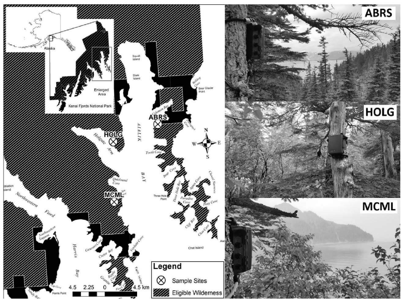
Figure 2. Examples of spectrograms with identified sound sources occurring in the Aialik Bay wilderness of Kenai Fjords National Park between June and September 2019.

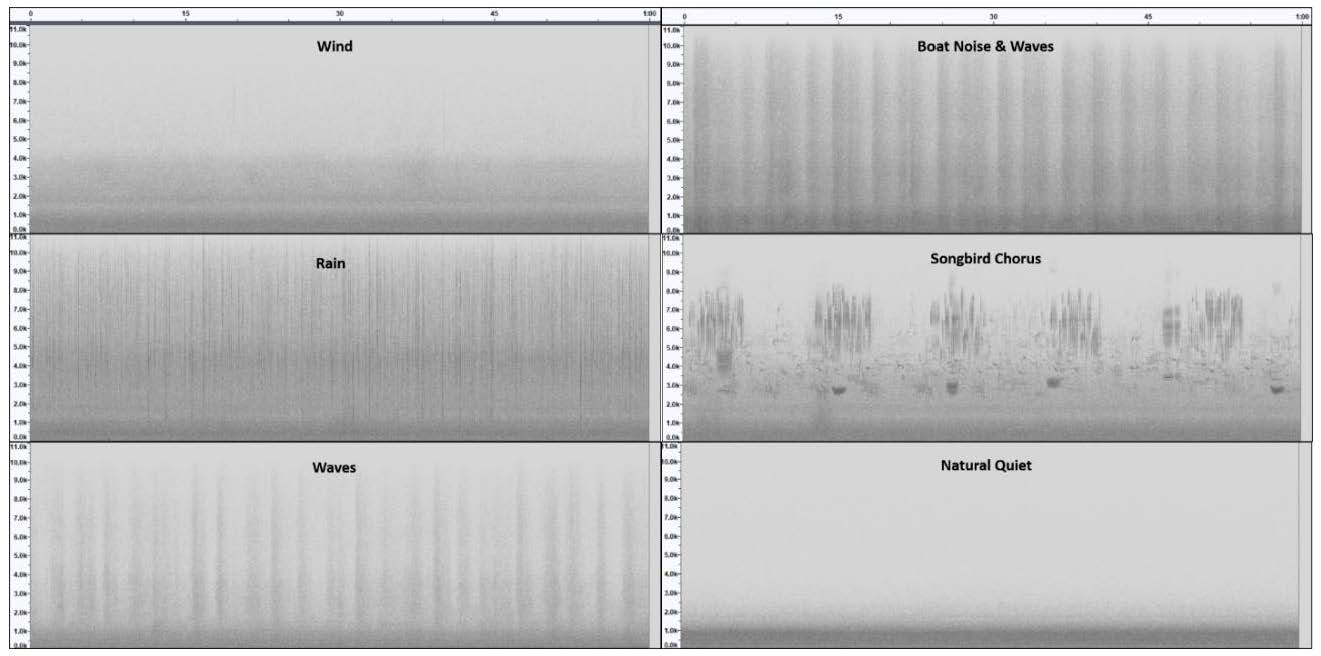
Figure 3. Frequency distribution of soundscape power (normalized watts/kHz) at three sound sampling sites in the eligible wilderness of Aialik Bay, Kenai Fjords National Park, Alaska from 26 June to 21 September 2019. Reference lines included are included for comparison.

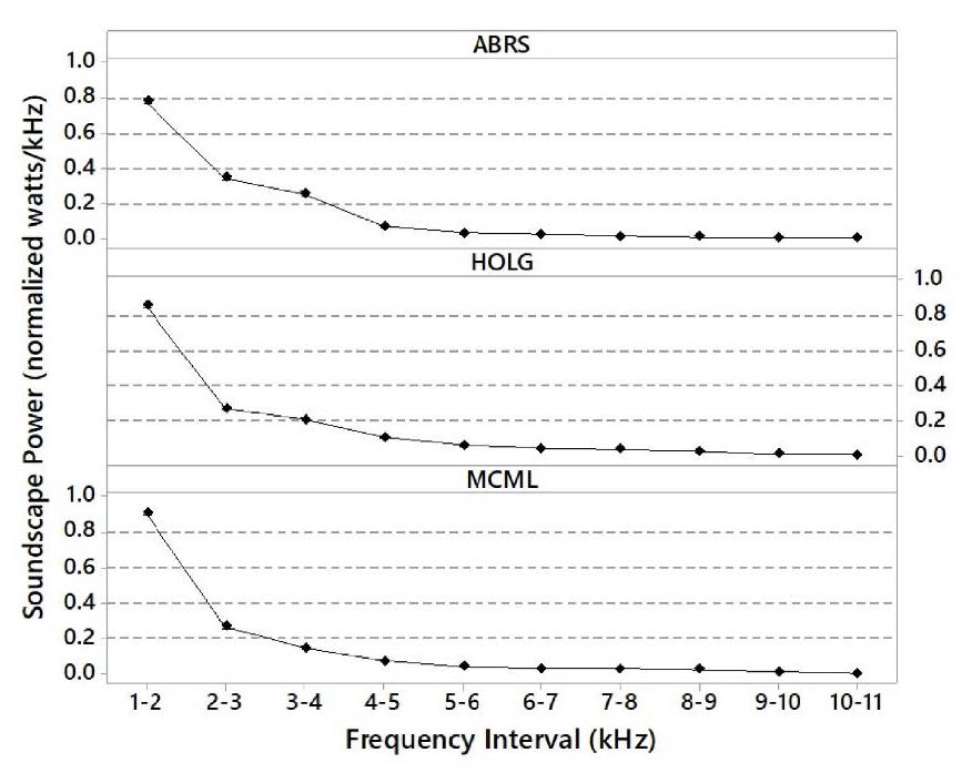
Figure 4. Temporal distribution of soundscape power (normalized watts/kHz) in the 1–2 kHz frequency interval by study day at three sample sites within the eligible wilderness of Aialik Bay, Kenai Fjords National Park, Alaska from 26 June to 21 September 2019 with thresholds of peak (>0.95 normalized watts/kHz) and minimum values (<0.6 normalized watts/kHz). Error bars represent 95% confidence intervals.

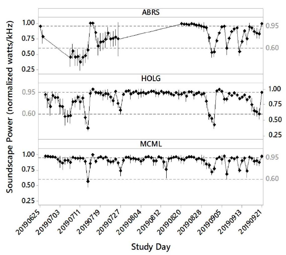
Figure 5. Proportion of sound sources occurring on study days with peak (>0.95 normalized watts/kHz) and minimum values (<0.60 normalized watts/kHz) of soundscape power in the 1–2 kHz frequency interval at three sample sites within the eligible wilderness of Aialik Bay, Kenai Fjords National Park, Alaska from 26 June to 21 September 2019.

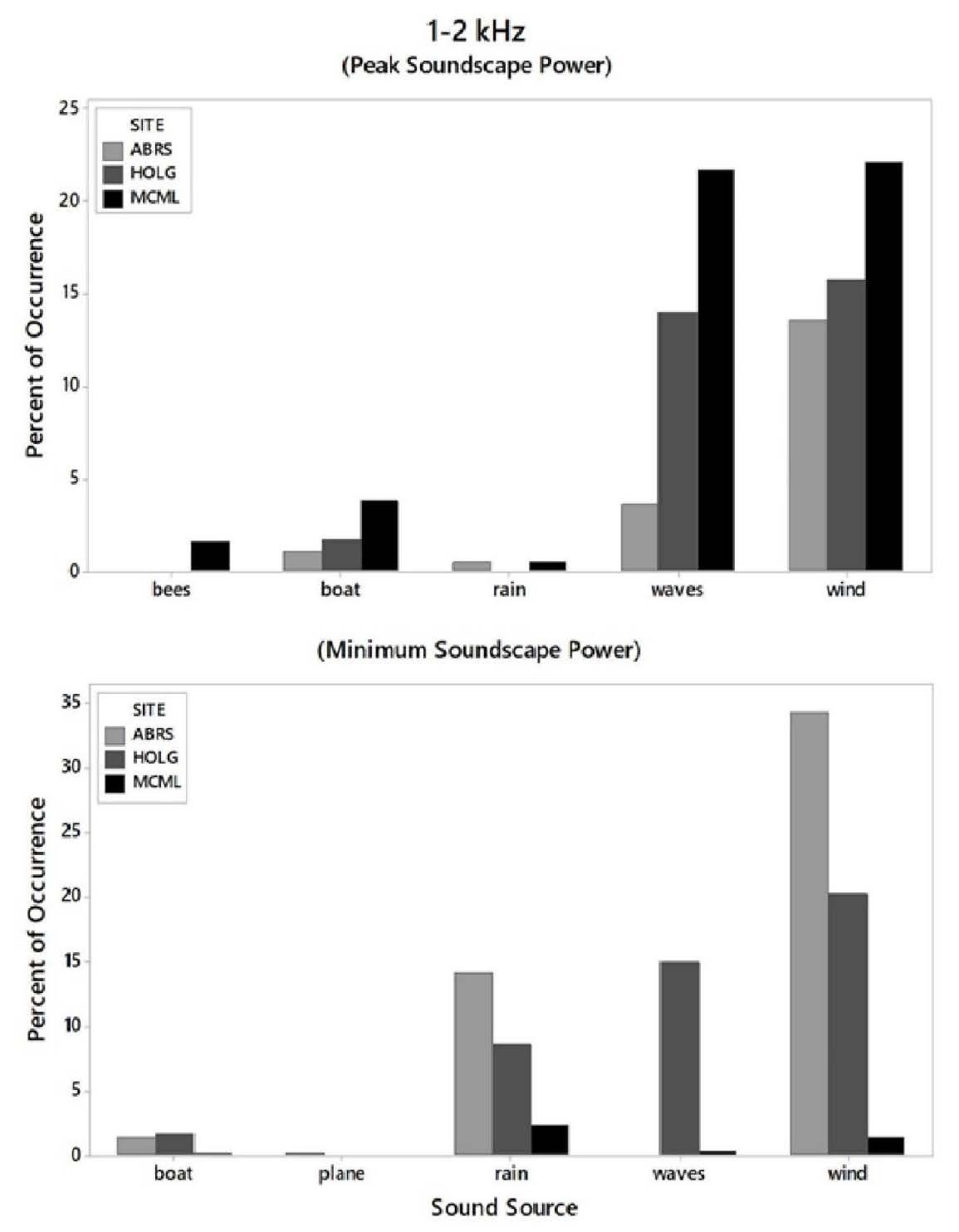
Figure 6. Temporal distribution of soundscape power (normalized watts/kHz) in the 2–5 kHz frequency interval by study day at three sample site within the eligible wilderness of Aialik Bay, Kenai Fjords National Park, Alaska from 26 June to 21 September 2019 with thresholds of peak (>0.30 normalized watts/kHz) and minimum (<0.10 normalized watts/kHz) values. Error bars represent 95% confidence intervals.

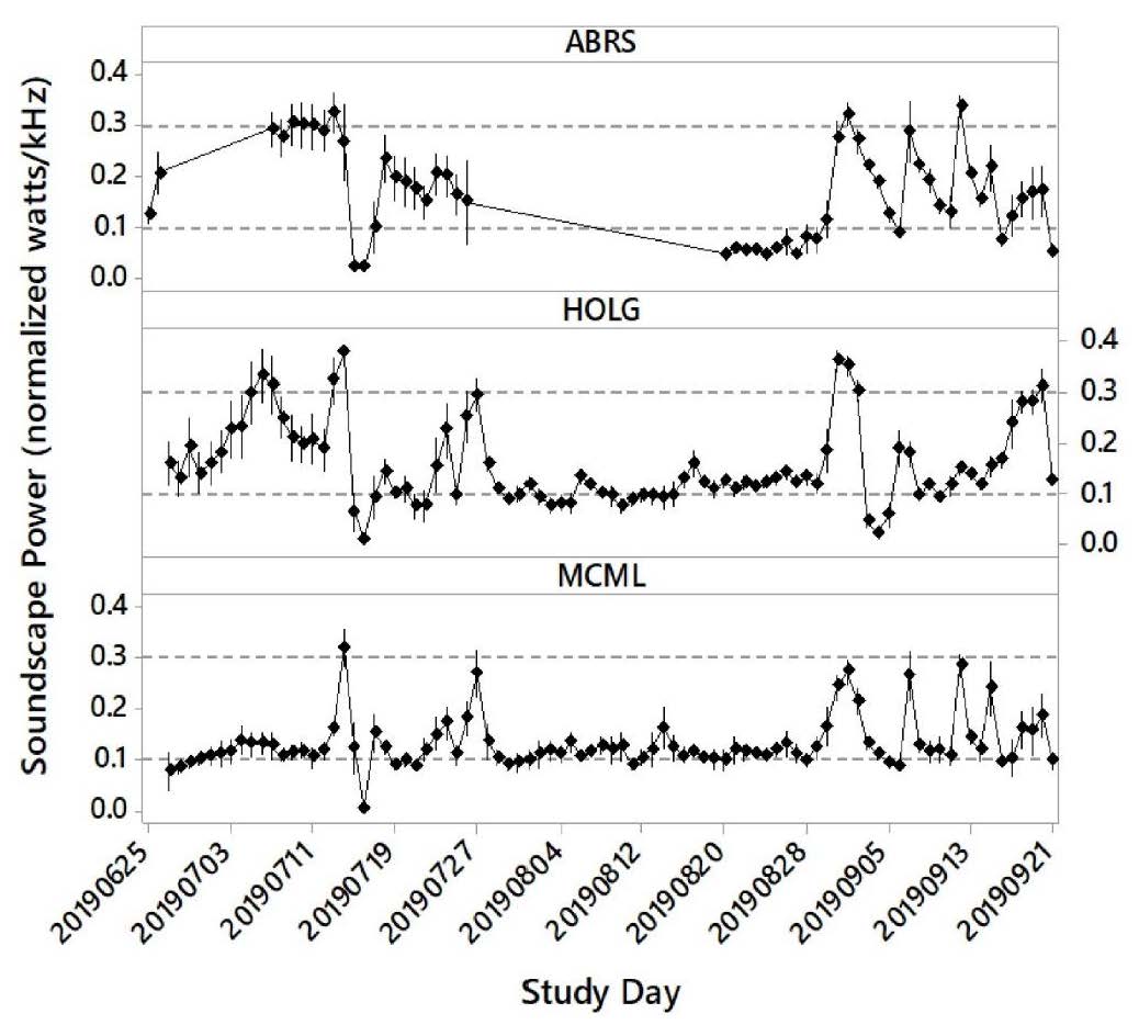
Figure 7. Proportion of sound sources occurring on study days with peak (>0.30 normalized watts/kHz) and minimum (<0.10 normalized watts/kHz) values of soundscape power in the 2–5 kHz frequency interval at three sample site within the eligible wilderness of Aialik Bay, Kenai Fjords National Park, Alaska from 26 June to 21 September 2019.

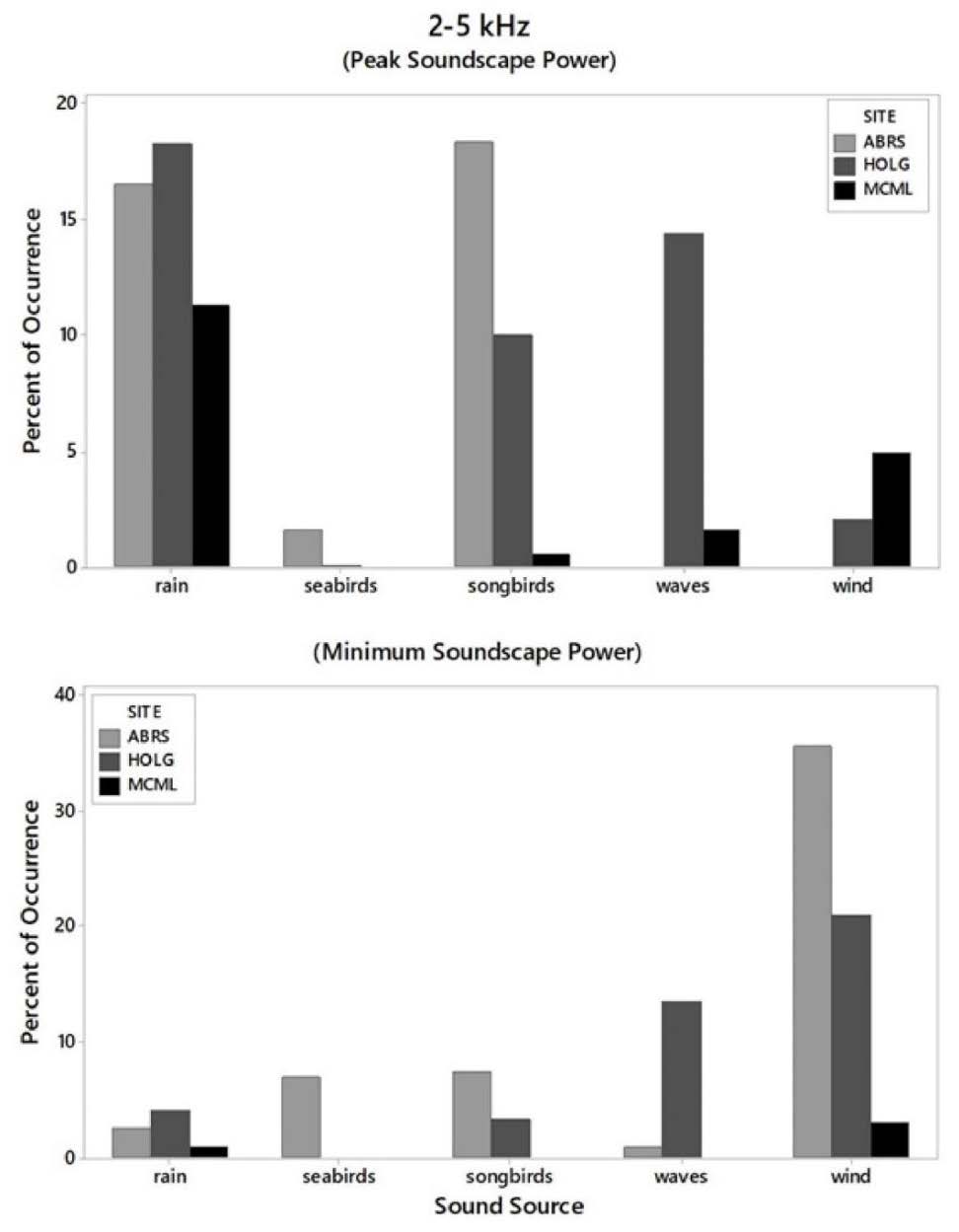
Figure 8. Temporal distribution of soundscape power (normalized watts/kHz) in the 1–2 kHz frequency interval by 24 h timeframes at three sample sites within the eligible wilderness of Aialik Bay, Kenai Fjords National Park, Alaska from 26 June to 21 September 2019. Error bars represent 95% confidence intervals. Y-axis labels are not scaled equally.

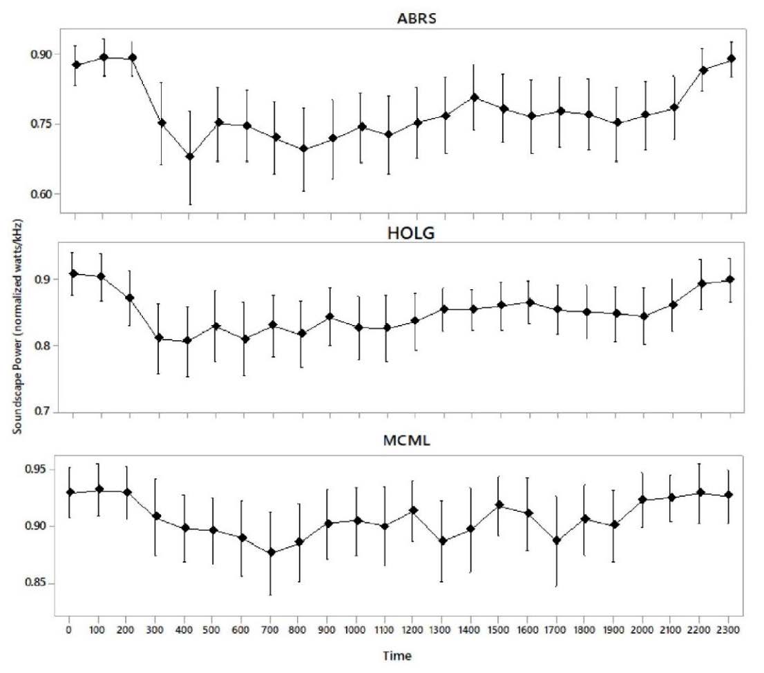
Figure 9. Temporal distribution of soundscape power (normalized watts/kHz) in the 2–5 kHz frequency interval by 24 h timeframes at three sample sites within the eligible wilderness of Aialik Bay, Kenai Fjords National Park, Alaska from 26 June to 21 September 2019. Error bars represent 95% confidence intervals. Y-axis labels are not scaled equally.

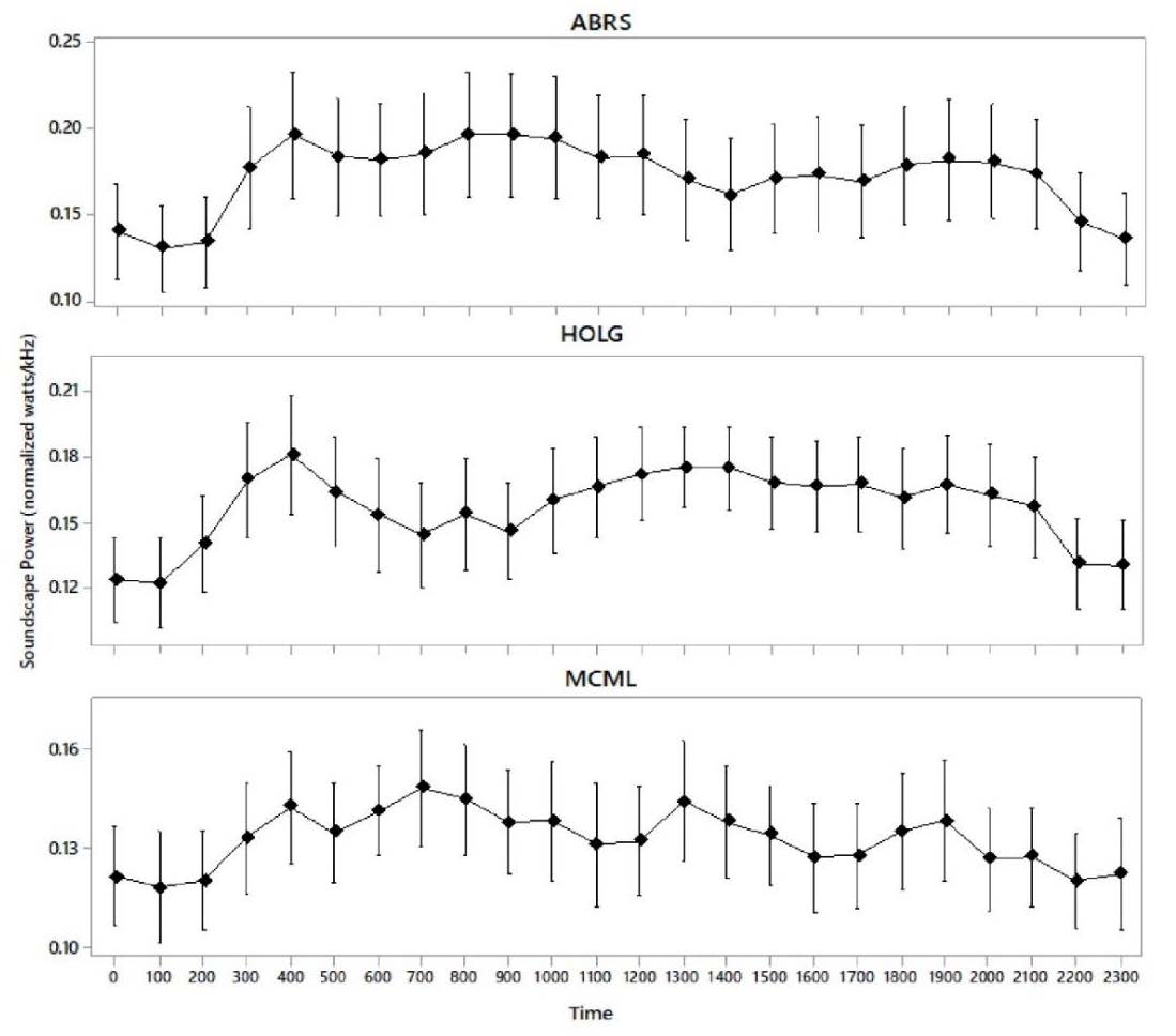
Figure 10. Temporal patterns of the Normalized Differential Soundscape Index (NDSI) by study day and 24 h timeframes at three sample sites within the eligible wilderness of Aialik Bay, Kenai Fjords National Park, Alaska from 26 June to 21 September 2019. Error bars represent 95% confidence intervals. Y-axis labels are not scaled equally.

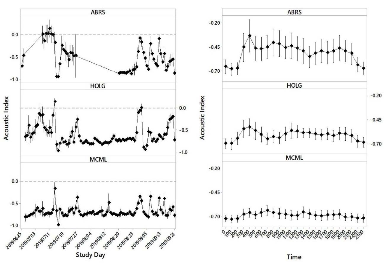
Table 1. Sound sample site names, geographic location (WGS84), and environmental characteristics in the eligible wilderness of Aialik Bay, Kenai Fjords National Park, Alaska from 27 June to 21 September 2019.

Site	Latitude	Longitude	Elevation (m)	Distance to Coast (m)	Habitat Type
ABRS	59.85183	−149.65599	47.2	86.2	Hemlock-subalpine meadow
HOLG	59.83416	−149.77020	9.7	15.7	Old-growth mixed-conifer forest
MCML	59.76077	−149.77730	19.5	13.5	Rocky mixed shrub-conifer forest

Journal of Ecoacoustics